TensorFlow 2.0 : 上級 Tutorials : 生成 :- Pix2Pix (翻訳/解説)
翻訳 : (株)クラスキャット セールスインフォメーション
作成日時 : 11/22/2019
* 本ページは、TensorFlow org サイトの TF 2.0 – Advanced Tutorials – Generative の以下のページを翻訳した上で
適宜、補足説明したものです:
* サンプルコードの動作確認はしておりますが、必要な場合には適宜、追加改変しています。
* ご自由にリンクを張って頂いてかまいませんが、sales-info@classcat.com までご一報いただけると嬉しいです。

- お住まいの地域に関係なく Web ブラウザからご参加頂けます。事前登録 が必要ですのでご注意ください。
- Windows PC のブラウザからご参加が可能です。スマートデバイスもご利用可能です。
◆ お問合せ : 本件に関するお問い合わせ先は下記までお願いいたします。
| 株式会社クラスキャット セールス・マーケティング本部 セールス・インフォメーション |
| E-Mail:sales-info@classcat.com ; WebSite: https://www.classcat.com/ |
| Facebook: https://www.facebook.com/ClassCatJP/ |
生成 :- Pix2Pix
このノートブックは Image-to-Image Translation with Conditional Adversarial Networks で記述されている、条件付き GAN を使用して画像から画像への変換を実演します。このテクニックを使用して白黒写真を彩色したり、google マップを google earth に変換する等のことができます。ここでは、建物の正面 (= facade) をリアルな建物に変換します。
サンプルでは、CMP Facade データベース を使用します、これは プラハの Czech Technical University の Center for Machine Perception により役立つように提供されています。サンプルを短く保つために、上の ペーパー の著者たちにより作成された、このデータセットの前処理された コピー を使用します。
各エポックは単一の V100 GPU 上で 15 秒前後かかります。
(訳注: Beta 版での記述によれば > 各エポックは単一の P100 GPU 上で 58 秒前後かかります。)
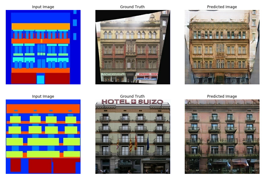
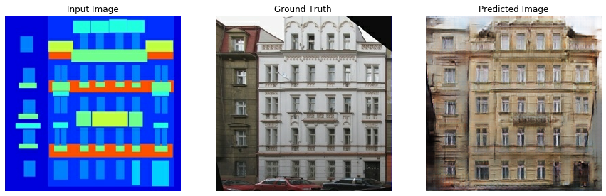
下は 200 エポックの間モデルを訓練した後に生成された出力です。
TensorFlow と他のライブラリをインポートする
from __future__ import absolute_import, division, print_function, unicode_literals

import tensorflow as tf

import os
import time

from matplotlib import pyplot as plt
from IPython import display
!pip install -q -U tensorboardデータセットをロードする データセットと類似のデータセットを ここ からダウンロードできます。(上の) ペーパーで言及されているように、訓練データセットにランダムに jittering とミラーリングを適用します。
- ランダム jittering では、画像は 286 x 286 にリサイズされてからランダムに 256 x 256 にクロップされます。
- ランダム・ミラーリングでは、画像は水平に i.e. 左から右にランダムにフリップ (反転) されます。
_URL = 'https://people.eecs.berkeley.edu/~tinghuiz/projects/pix2pix/datasets/facades.tar.gz'

path_to_zip = tf.keras.utils.get_file('facades.tar.gz',
                                      origin=_URL,
                                      extract=True)

PATH = os.path.join(os.path.dirname(path_to_zip), 'facades/')
Downloading data from https://people.eecs.berkeley.edu/~tinghuiz/projects/pix2pix/datasets/facades.tar.gz
30171136/30168306 [==============================] - 2s 0us/step
BUFFER_SIZE = 400
BATCH_SIZE = 1
IMG_WIDTH = 256
IMG_HEIGHT = 256
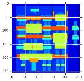
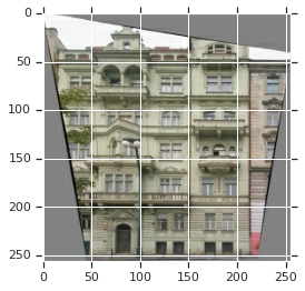
def load(image_file):
  image = tf.io.read_file(image_file)
  image = tf.image.decode_jpeg(image)

  w = tf.shape(image)[1]

  w = w // 2
  real_image = image[:, :w, :]
  input_image = image[:, w:, :]

  input_image = tf.cast(input_image, tf.float32)
  real_image = tf.cast(real_image, tf.float32)

  return input_image, real_image
inp, re = load(PATH+'train/100.jpg')
# casting to int for matplotlib to show the image
plt.figure()
plt.imshow(inp/255.0)
plt.figure()
plt.imshow(re/255.0)
<matplotlib.image.AxesImage at 0x7ff6617e4898>
def resize(input_image, real_image, height, width):
  input_image = tf.image.resize(input_image, [height, width],
                                method=tf.image.ResizeMethod.NEAREST_NEIGHBOR)
  real_image = tf.image.resize(real_image, [height, width],
                               method=tf.image.ResizeMethod.NEAREST_NEIGHBOR)

  return input_image, real_image
def random_crop(input_image, real_image):
  stacked_image = tf.stack([input_image, real_image], axis=0)
  cropped_image = tf.image.random_crop(
      stacked_image, size=[2, IMG_HEIGHT, IMG_WIDTH, 3])

  return cropped_image[0], cropped_image[1]
# normalizing the images to [-1, 1]

def normalize(input_image, real_image):
  input_image = (input_image / 127.5) - 1
  real_image = (real_image / 127.5) - 1

  return input_image, real_image
@tf.function()
def random_jitter(input_image, real_image):
  # resizing to 286 x 286 x 3
  input_image, real_image = resize(input_image, real_image, 286, 286)

  # randomly cropping to 256 x 256 x 3
  input_image, real_image = random_crop(input_image, real_image)

  if tf.random.uniform(()) > 0.5:
    # random mirroring
    input_image = tf.image.flip_left_right(input_image)
    real_image = tf.image.flip_left_right(real_image)

  return input_image, real_image
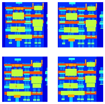
下の画像で画像がランダム jittering を通り抜けているのを見ることができます。ペーパーで記述されているランダム jittering は以下を行なうためです :
- 画像をより大きい高さと幅にリサイズします
- ランダムにターゲットサイズにクロップします
- ランダムに画像を水平に反転します
plt.figure(figsize=(6, 6))
for i in range(4):
  rj_inp, rj_re = random_jitter(inp, re)
  plt.subplot(2, 2, i+1)
  plt.imshow(rj_inp/255.0)
  plt.axis('off')
plt.show()
def load_image_train(image_file):
  input_image, real_image = load(image_file)
  input_image, real_image = random_jitter(input_image, real_image)
  input_image, real_image = normalize(input_image, real_image)

  return input_image, real_image
def load_image_test(image_file):
  input_image, real_image = load(image_file)
  input_image, real_image = resize(input_image, real_image,
                                   IMG_HEIGHT, IMG_WIDTH)
  input_image, real_image = normalize(input_image, real_image)

  return input_image, real_image
入力パイプライン
train_dataset = tf.data.Dataset.list_files(PATH+'train/*.jpg')
train_dataset = train_dataset.map(load_image_train,
                                  num_parallel_calls=tf.data.experimental.AUTOTUNE)
train_dataset = train_dataset.shuffle(BUFFER_SIZE)
train_dataset = train_dataset.batch(BATCH_SIZE)
test_dataset = tf.data.Dataset.list_files(PATH+'test/*.jpg')
test_dataset = test_dataset.map(load_image_test)
test_dataset = test_dataset.batch(BATCH_SIZE)
Generator を構築する
- generator のアーキテクチャは変更された U-Net です。
- エンコーダの各ブロックは (Conv -> Batchnorm -> Leaky ReLU)
- デコーダの各ブロックは (Transposed Conv -> Batchnorm -> Dropout(applied to the first 3 blocks) -> ReLU)
- エンコーダとデコーダの間に (U-Net 内のように) スキップ接続があります。
OUTPUT_CHANNELS = 3
def downsample(filters, size, apply_batchnorm=True):
  initializer = tf.random_normal_initializer(0., 0.02)

  result = tf.keras.Sequential()
  result.add(
      tf.keras.layers.Conv2D(filters, size, strides=2, padding='same',
                             kernel_initializer=initializer, use_bias=False))

  if apply_batchnorm:
    result.add(tf.keras.layers.BatchNormalization())

  result.add(tf.keras.layers.LeakyReLU())

  return result
down_model = downsample(3, 4)
down_result = down_model(tf.expand_dims(inp, 0))
print (down_result.shape)
(1, 128, 128, 3)
def upsample(filters, size, apply_dropout=False):
  initializer = tf.random_normal_initializer(0., 0.02)

  result = tf.keras.Sequential()
  result.add(
    tf.keras.layers.Conv2DTranspose(filters, size, strides=2,
                                    padding='same',
                                    kernel_initializer=initializer,
                                    use_bias=False))

  result.add(tf.keras.layers.BatchNormalization())

  if apply_dropout:
      result.add(tf.keras.layers.Dropout(0.5))

  result.add(tf.keras.layers.ReLU())

  return result
up_model = upsample(3, 4)
up_result = up_model(down_result)
print (up_result.shape)
(1, 256, 256, 3)
def Generator():
  inputs = tf.keras.layers.Input(shape=[256,256,3])

  down_stack = [
    downsample(64, 4, apply_batchnorm=False), # (bs, 128, 128, 64)
    downsample(128, 4), # (bs, 64, 64, 128)
    downsample(256, 4), # (bs, 32, 32, 256)
    downsample(512, 4), # (bs, 16, 16, 512)
    downsample(512, 4), # (bs, 8, 8, 512)
    downsample(512, 4), # (bs, 4, 4, 512)
    downsample(512, 4), # (bs, 2, 2, 512)
    downsample(512, 4), # (bs, 1, 1, 512)
  ]

  up_stack = [
    upsample(512, 4, apply_dropout=True), # (bs, 2, 2, 1024)
    upsample(512, 4, apply_dropout=True), # (bs, 4, 4, 1024)
    upsample(512, 4, apply_dropout=True), # (bs, 8, 8, 1024)
    upsample(512, 4), # (bs, 16, 16, 1024)
    upsample(256, 4), # (bs, 32, 32, 512)
    upsample(128, 4), # (bs, 64, 64, 256)
    upsample(64, 4), # (bs, 128, 128, 128)
  ]

  initializer = tf.random_normal_initializer(0., 0.02)
  last = tf.keras.layers.Conv2DTranspose(OUTPUT_CHANNELS, 4,
                                         strides=2,
                                         padding='same',
                                         kernel_initializer=initializer,
                                         activation='tanh') # (bs, 256, 256, 3)

  x = inputs

  # Downsampling through the model
  skips = []
  for down in down_stack:
    x = down(x)
    skips.append(x)

  skips = reversed(skips[:-1])

  # Upsampling and establishing the skip connections
  for up, skip in zip(up_stack, skips):
    x = up(x)
    x = tf.keras.layers.Concatenate()([x, skip])

  x = last(x)

  return tf.keras.Model(inputs=inputs, outputs=x)
generator = Generator()
tf.keras.utils.plot_model(generator, show_shapes=True, dpi=64)

gen_output = generator(inp[tf.newaxis,...], training=False)
plt.imshow(gen_output[0,...])
Clipping input data to the valid range for imshow with RGB data ([0..1] for floats or [0..255] for integers).

<matplotlib.image.AxesImage at 0x7ff5d87565c0>
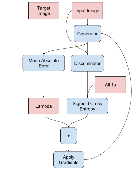
- Generator 損失
generator の訓練手続きは下で示されます :
LAMBDA = 100
def generator_loss(disc_generated_output, gen_output, target):
  gan_loss = loss_object(tf.ones_like(disc_generated_output), disc_generated_output)

  # mean absolute error
  l1_loss = tf.reduce_mean(tf.abs(target - gen_output))

  total_gen_loss = gan_loss + (LAMBDA * l1_loss)

  return total_gen_loss, gan_loss, l1_loss
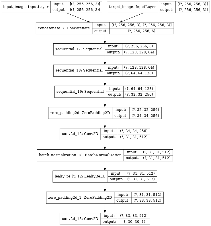
Discriminator を構築する
- discriminator は PatchGAN です。
- discriminator の各ブロックは (Conv -> BatchNorm -> Leaky ReLU) です。
- 最後の層の後の出力の shape は (batch_size, 30, 30, 1) です。
- 出力の各 30x30 パッチが入力画像の 70x70 の断片を分類します (そのようなアーキテクチャは PatchGAN と呼ばれます)。
- discriminator は 2 つの入力を受け取ります。
- 入力画像とターゲット画像、これは real として分類するべきです。
- 入力画像と生成画像 (generator の出力)、これは fake として分類するべきです。
- これらの 2 つの入力をコード (tf.concat([inp, tar], axis=-1)) で一緒に結合します。
def Discriminator():
  initializer = tf.random_normal_initializer(0., 0.02)

  inp = tf.keras.layers.Input(shape=[256, 256, 3], name='input_image')
  tar = tf.keras.layers.Input(shape=[256, 256, 3], name='target_image')

  x = tf.keras.layers.concatenate([inp, tar]) # (bs, 256, 256, channels*2)

  down1 = downsample(64, 4, False)(x) # (bs, 128, 128, 64)
  down2 = downsample(128, 4)(down1) # (bs, 64, 64, 128)
  down3 = downsample(256, 4)(down2) # (bs, 32, 32, 256)

  zero_pad1 = tf.keras.layers.ZeroPadding2D()(down3) # (bs, 34, 34, 256)
  conv = tf.keras.layers.Conv2D(512, 4, strides=1,
                                kernel_initializer=initializer,
                                use_bias=False)(zero_pad1) # (bs, 31, 31, 512)

  batchnorm1 = tf.keras.layers.BatchNormalization()(conv)

  leaky_relu = tf.keras.layers.LeakyReLU()(batchnorm1)

  zero_pad2 = tf.keras.layers.ZeroPadding2D()(leaky_relu) # (bs, 33, 33, 512)

  last = tf.keras.layers.Conv2D(1, 4, strides=1,
                                kernel_initializer=initializer)(zero_pad2) # (bs, 30, 30, 1)

  return tf.keras.Model(inputs=[inp, tar], outputs=last)
discriminator = Discriminator()
tf.keras.utils.plot_model(discriminator, show_shapes=True, dpi=64)
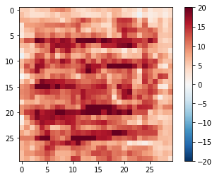
disc_out = discriminator([inp[tf.newaxis,...], gen_output], training=False)
plt.imshow(disc_out[0,...,-1], vmin=-20, vmax=20, cmap='RdBu_r')
plt.colorbar()
<matplotlib.colorbar.Colorbar at 0x7ff5d84dcf28>

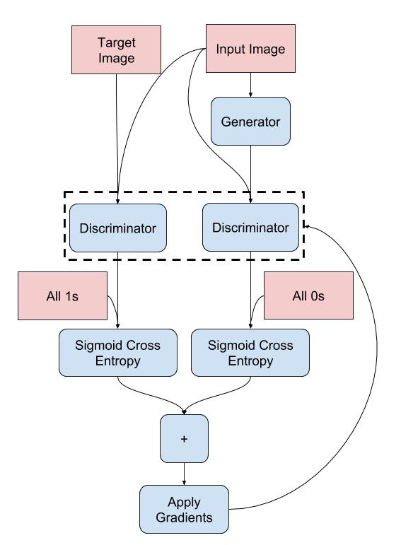
- Discriminator 損失
- discriminator 損失関数は 2 つの入力を取ります; real 画像、生成画像 です。
- real_loss は real 画像 と 1 の配列 (何故ならばこれらは real 画像だからです) の sigmod 交差エントロピー損失です。
- generated_loss は 生成画像 と ゼロの配列 (何故ならばこれらは fake 画像だからです) の sigmod 交差エントロピー損失です。
- それから total_loss は real_loss と generated_loss の合計です。
loss_object = tf.keras.losses.BinaryCrossentropy(from_logits=True)
def discriminator_loss(disc_real_output, disc_generated_output):
  real_loss = loss_object(tf.ones_like(disc_real_output), disc_real_output)

  generated_loss = loss_object(tf.zeros_like(disc_generated_output), disc_generated_output)

  total_disc_loss = real_loss + generated_loss

  return total_disc_loss
discriminator のための訓練手続きは下で示されます。
アーキテクチャとハイパーパラメータについて更に学習するためには、ペーパー を参照できます。
損失関数と Optimizer とチェックポイント・セーバーを定義する
generator_optimizer = tf.keras.optimizers.Adam(2e-4, beta_1=0.5)
discriminator_optimizer = tf.keras.optimizers.Adam(2e-4, beta_1=0.5)
checkpoint_dir = './training_checkpoints'
checkpoint_prefix = os.path.join(checkpoint_dir, "ckpt")
checkpoint = tf.train.Checkpoint(generator_optimizer=generator_optimizer,
                                 discriminator_optimizer=discriminator_optimizer,
                                 generator=generator,
                                 discriminator=discriminator)
チェックポイント (オブジェクトベースのセーブ)
checkpoint_dir = './training_checkpoints'
checkpoint_prefix = os.path.join(checkpoint_dir, "ckpt")
checkpoint = tf.train.Checkpoint(generator_optimizer=generator_optimizer,
                                 discriminator_optimizer=discriminator_optimizer,
                                 generator=generator,
                                 discriminator=discriminator)
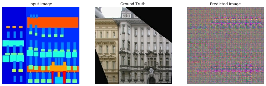
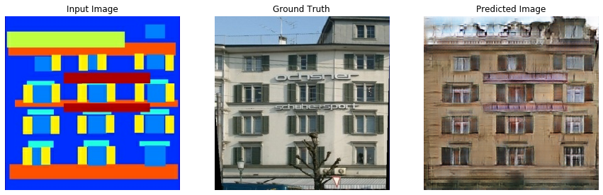
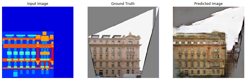
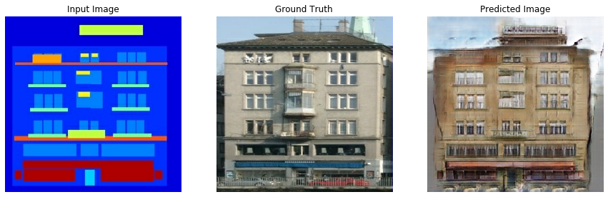
画像を生成する
訓練の間に幾つかの画像をプロットするための関数を書きます。
- テスト・データセットから generator に画像を渡します。
- それから generator は入力画像を出力に変換します。
- 最後のステップは予測をプロットすることです、そして voila !
★ Note: training=True はここでは意図的です、何故ならばテストデータセット上でモデルを実行する間バッチ統計を望むからです。training=False を使用する場合、訓練データセットから学習された累積統計を得ます (それは私達は望みません)。
def generate_images(model, test_input, tar):
  prediction = model(test_input, training=True)
  plt.figure(figsize=(15,15))

  display_list = [test_input[0], tar[0], prediction[0]]
  title = ['Input Image', 'Ground Truth', 'Predicted Image']

  for i in range(3):
    plt.subplot(1, 3, i+1)
    plt.title(title[i])
    # getting the pixel values between [0, 1] to plot it.
    plt.imshow(display_list[i] * 0.5 + 0.5)
    plt.axis('off')
  plt.show()
for example_input, example_target in test_dataset.take(1):
  generate_images(generator, example_input, example_target)
訓練
- 各サンプル入力に対して出力を生成します。
- discriminator は最初の入力として input_image と生成画像を受け取ります。2 番目の入力は input_image と target_image です。
- 次に generator と discriminator 損失を計算します。
- それから、generator と discriminator 変数 (入力) の両者に関する損失の勾配を計算してそれらを optimizer に適用します。
- それから損失を TensorBoard に記録します。
EPOCHS = 150
import datetime
log_dir="logs/"

summary_writer = tf.summary.create_file_writer(
  log_dir + "fit/" + datetime.datetime.now().strftime("%Y%m%d-%H%M%S"))
@tf.function
def train_step(input_image, target, epoch):
  with tf.GradientTape() as gen_tape, tf.GradientTape() as disc_tape:
    gen_output = generator(input_image, training=True)

    disc_real_output = discriminator([input_image, target], training=True)
    disc_generated_output = discriminator([input_image, gen_output], training=True)

    gen_total_loss, gen_gan_loss, gen_l1_loss = generator_loss(disc_generated_output, gen_output, target)
    disc_loss = discriminator_loss(disc_real_output, disc_generated_output)

  generator_gradients = gen_tape.gradient(gen_total_loss,
                                          generator.trainable_variables)
  discriminator_gradients = disc_tape.gradient(disc_loss,
                                               discriminator.trainable_variables)

  generator_optimizer.apply_gradients(zip(generator_gradients,
                                          generator.trainable_variables))
  discriminator_optimizer.apply_gradients(zip(discriminator_gradients,
                                              discriminator.trainable_variables))

  with summary_writer.as_default():
    tf.summary.scalar('gen_total_loss', gen_total_loss, step=epoch)
    tf.summary.scalar('gen_gan_loss', gen_gan_loss, step=epoch)
    tf.summary.scalar('gen_l1_loss', gen_l1_loss, step=epoch)
    tf.summary.scalar('disc_loss', disc_loss, step=epoch)
実際の訓練ループは :
- エポック数に渡り反復します。
- 各エポックで、それは表示をクリアして、その進捗を示すために generate_images を実行します。
- 各エポックで、それは訓練データセットに渡り反復し、各サンプルのために '.' をプリントします。
- それは 20 エポック毎にチェックポイントをセーブします。
def fit(train_ds, epochs, test_ds):
  for epoch in range(epochs):
    start = time.time()

    display.clear_output(wait=True)

    for example_input, example_target in test_ds.take(1):
      generate_images(generator, example_input, example_target)
    print("Epoch: ", epoch)

    # Train
    for n, (input_image, target) in train_ds.enumerate():
      print('.', end='')
      if (n+1) % 100 == 0:
        print()
      train_step(input_image, target, epoch)
    print()

    # saving (checkpoint) the model every 20 epochs
    if (epoch + 1) % 20 == 0:
      checkpoint.save(file_prefix = checkpoint_prefix)

    print ('Time taken for epoch {} is {} sec\n'.format(epoch + 1,
                                                        time.time()-start))
  checkpoint.save(file_prefix = checkpoint_prefix)
この訓練ループは訓練進捗を監視するために TensorBoard で容易に見ることができるログをセーブします。ローカルで作業するときには別の tensorboard プロセスを起動します。ノートブックでは、TensorBoard で監視することを望む場合、訓練を始める前に viewer を起動するのが最も容易です。
viewer を起動するには次をコードセルにペーストしてください :
%load_ext tensorboard
%tensorboard --logdir {log_dir}
今は訓練ループを実行します :
fit(train_dataset, EPOCHS, test_dataset)
Epoch:  140
............................................................
TensorBoard の結果を公に共有することを望む場合次をコードセルにコピーすることによりログを TensorBoard.dev にアップロードできます。
★ Note: これは Google アカウントを必要とします。
!tensorboard dev upload --logdir {log_dir}
このノートブックの 前の実行の結果 を TensorBoard.dev で見ることができます。
TensorBoard.dev はホスティング、追跡そして ML 実験の皆との共有のための managed experience です。
それはまた <iframe> を使用してインラインで含むこともできます :
display.IFrame(
    src="https://tensorboard.dev/experiment/lZ0C6FONROaUMfjYkVyJqw",
    width="100%",
    height="1000px")
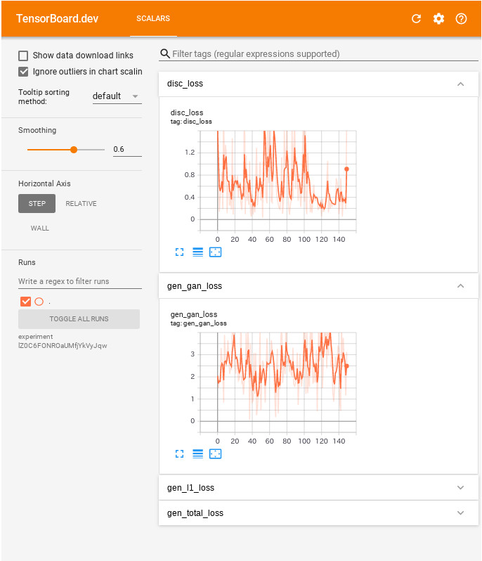
GAN からのログの解釈は単純な分類や回帰モデルよりも微妙です。探すべきものは ::
- いずれのモデルも「勝利」していないことを確認してください。gen_gan_loss か disc_loss のいずれかが非常に低い場合、このモデルは他を支配している指標で、結合されたモデルを成功的に訓練していません。
- それらの損失のために値 log(2) = 0.69 は良い参照ポイントです、何故ならばそれは 2 の perplexity を示すからです。That the discriminator is on average equally uncertain about the two options.
- disc_loss について 0.69 より下の値はリアル+生成画像の結合セット上、discriminator がランダムよりも上手くやっていることを意味します。
- gen_gan_loss について 0.69 よりも下の値は generator が discriminator を騙す点でランダムよりも上手くやっていることを意味します。
- 訓練が進むにつれて gen_l1_loss は下がるはずです。
最新のチェックポイントをリストアしてテストする
!ls {checkpoint_dir}
checkpoint          ckpt-5.data-00000-of-00002
ckpt-1.data-00000-of-00002  ckpt-5.data-00001-of-00002
ckpt-1.data-00001-of-00002  ckpt-5.index
ckpt-1.index            ckpt-6.data-00000-of-00002
ckpt-2.data-00000-of-00002  ckpt-6.data-00001-of-00002
ckpt-2.data-00001-of-00002  ckpt-6.index
ckpt-2.index            ckpt-7.data-00000-of-00002
ckpt-3.data-00000-of-00002  ckpt-7.data-00001-of-00002
ckpt-3.data-00001-of-00002  ckpt-7.index
ckpt-3.index            ckpt-8.data-00000-of-00002
ckpt-4.data-00000-of-00002  ckpt-8.data-00001-of-00002
ckpt-4.data-00001-of-00002  ckpt-8.index
ckpt-4.index
# restoring the latest checkpoint in checkpoint_dir
checkpoint.restore(tf.train.latest_checkpoint(checkpoint_dir))
<tensorflow.python.training.tracking.util.CheckpointLoadStatus at 0x7ff04ea33588>
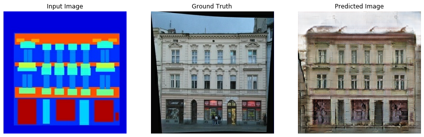
テスト・データセットを使用して生成する
# Run the trained model on a few examples from the test dataset
for inp, tar in test_dataset.take(5):
  generate_images(generator, inp, tar)

以上