Keras 2 : examples : 積分勾配によるモデル解釈 (翻訳/解説)

翻訳 : (株)クラスキャット セールスインフォメーション
作成日時 : 11/24/2021 (keras 2.7.0)

* 本ページは、Keras の以下のドキュメントを翻訳した上で適宜、補足説明したものです：

• Code examples : Computer Vision : Model interpretability with Integrated Gradients (Author: A_K_Nain)

* サンプルコードの動作確認はしておりますが、必要な場合には適宜、追加改変しています。
* ご自由にリンクを張って頂いてかまいませんが、sales-info@classcat.com までご一報いただけると嬉しいです。

Keras 2 : examples : 積分勾配によるモデル解釈

Description: 分類モデルのために積分勾配をどのように取得するか。

積分勾配

積分勾配 (Integrated Gradients) は分類モデルの予測をその入力特徴に帰着させるためのテクニックです。それはモデル解釈テクニックです : それを入力特徴とモデル予測の間の関係を可視化するために使用できます。

積分勾配は入力の特徴に関する予測の勾配を計算することについてのバリエーションです。積分勾配を計算するために、以下のステップを実行する必要があります :

1. 入力と出力を識別します。私達のケースでは、入力は画像で出力はモデルの最後の層 (softmax 活性を持つ dense 層) です。
   

2. 特定のデータポイント上で予測を行なうとき、どの特徴がニューラルネットワークに対して重要であるかを計算します。これらの特徴を識別するために、ベースライン入力を選択する必要があります。ベースライン入力はブラック画像 (総てのピクセル値をゼロに設定) やランダムノイズであることが可能です。ベースライン入力の shape は入力画像, e.g. (299, 299, 3) と同じである必要があります。
   

3. 与えられた数のステップに対してベースラインを補間します。ステップ数は与えられた入力画像に対する勾配近似で必要なステップを表します。ステップ数はハイパーパラメータです。著者は 20 と 1000 ステップの間の任意の値を使用することを勧めています。
   

4. これらの補間された画像を前処理して forward パスを実行します。
   

5. これらの補間された画像に対する勾配を得ます。
   

6. 台形公式 (= trapezoidal rule) を使用して勾配積分 (= gradients integral) を近似します。

積分勾配についての詳細とこの方法が何故機能するかを読むためには、この優れた 記事 を読むことを考えてください。

リファレンス :

• 積分勾配原著 論文
• オリジナル実装

セットアップ

import numpy as np
import matplotlib.pyplot as plt
from scipy import ndimage
from IPython.display import Image

import tensorflow as tf
from tensorflow import keras
from tensorflow.keras import layers
from tensorflow.keras.applications import xception

# Size of the input image
img_size = (299, 299, 3)

# Load Xception model with imagenet weights
model = xception.Xception(weights="imagenet")

# The local path to our target image
img_path = keras.utils.get_file("elephant.jpg", "https://i.imgur.com/Bvro0YD.png")
display(Image(img_path))

Downloading data from https://i.imgur.com/Bvro0YD.png
4218880/4217496 [==============================] - 0s 0us/step

積分勾配アルゴリズム

def get_img_array(img_path, size=(299, 299)):
    # `img` is a PIL image of size 299x299
    img = keras.preprocessing.image.load_img(img_path, target_size=size)
    # `array` is a float32 Numpy array of shape (299, 299, 3)
    array = keras.preprocessing.image.img_to_array(img)
    # We add a dimension to transform our array into a "batch"
    # of size (1, 299, 299, 3)
    array = np.expand_dims(array, axis=0)
    return array


def get_gradients(img_input, top_pred_idx):
    """Computes the gradients of outputs w.r.t input image.

    Args:
        img_input: 4D image tensor
        top_pred_idx: Predicted label for the input image

    Returns:
        Gradients of the predictions w.r.t img_input
    """
    images = tf.cast(img_input, tf.float32)

    with tf.GradientTape() as tape:
        tape.watch(images)
        preds = model(images)
        top_class = preds[:, top_pred_idx]

    grads = tape.gradient(top_class, images)
    return grads


def get_integrated_gradients(img_input, top_pred_idx, baseline=None, num_steps=50):
    """Computes Integrated Gradients for a predicted label.

    Args:
        img_input (ndarray): Original image
        top_pred_idx: Predicted label for the input image
        baseline (ndarray): The baseline image to start with for interpolation
        num_steps: Number of interpolation steps between the baseline
            and the input used in the computation of integrated gradients. These
            steps along determine the integral approximation error. By default,
            num_steps is set to 50.

    Returns:
        Integrated gradients w.r.t input image
    """
    # If baseline is not provided, start with a black image
    # having same size as the input image.
    if baseline is None:
        baseline = np.zeros(img_size).astype(np.float32)
    else:
        baseline = baseline.astype(np.float32)

    # 1. Do interpolation.
    img_input = img_input.astype(np.float32)
    interpolated_image = [
        baseline + (step / num_steps) * (img_input - baseline)
        for step in range(num_steps + 1)
    ]
    interpolated_image = np.array(interpolated_image).astype(np.float32)

    # 2. Preprocess the interpolated images
    interpolated_image = xception.preprocess_input(interpolated_image)

    # 3. Get the gradients
    grads = []
    for i, img in enumerate(interpolated_image):
        img = tf.expand_dims(img, axis=0)
        grad = get_gradients(img, top_pred_idx=top_pred_idx)
        grads.append(grad[0])
    grads = tf.convert_to_tensor(grads, dtype=tf.float32)

    # 4. Approximate the integral using the trapezoidal rule
    grads = (grads[:-1] + grads[1:]) / 2.0
    avg_grads = tf.reduce_mean(grads, axis=0)

    # 5. Calculate integrated gradients and return
    integrated_grads = (img_input - baseline) * avg_grads
    return integrated_grads


def random_baseline_integrated_gradients(
    img_input, top_pred_idx, num_steps=50, num_runs=2
):
    """Generates a number of random baseline images.

    Args:
        img_input (ndarray): 3D image
        top_pred_idx: Predicted label for the input image
        num_steps: Number of interpolation steps between the baseline
            and the input used in the computation of integrated gradients. These
            steps along determine the integral approximation error. By default,
            num_steps is set to 50.
        num_runs: number of baseline images to generate

    Returns:
        Averaged integrated gradients for `num_runs` baseline images
    """
    # 1. List to keep track of Integrated Gradients (IG) for all the images
    integrated_grads = []

    # 2. Get the integrated gradients for all the baselines
    for run in range(num_runs):
        baseline = np.random.random(img_size) * 255
        igrads = get_integrated_gradients(
            img_input=img_input,
            top_pred_idx=top_pred_idx,
            baseline=baseline,
            num_steps=num_steps,
        )
        integrated_grads.append(igrads)

    # 3. Return the average integrated gradients for the image
    integrated_grads = tf.convert_to_tensor(integrated_grads)
    return tf.reduce_mean(integrated_grads, axis=0)

勾配と積分勾配を可視化するヘルパークラス

class GradVisualizer:
    """Plot gradients of the outputs w.r.t an input image."""

    def __init__(self, positive_channel=None, negative_channel=None):
        if positive_channel is None:
            self.positive_channel = [0, 255, 0]
        else:
            self.positive_channel = positive_channel

        if negative_channel is None:
            self.negative_channel = [255, 0, 0]
        else:
            self.negative_channel = negative_channel

    def apply_polarity(self, attributions, polarity):
        if polarity == "positive":
            return np.clip(attributions, 0, 1)
        else:
            return np.clip(attributions, -1, 0)

    def apply_linear_transformation(
        self,
        attributions,
        clip_above_percentile=99.9,
        clip_below_percentile=70.0,
        lower_end=0.2,
    ):
        # 1. Get the thresholds
        m = self.get_thresholded_attributions(
            attributions, percentage=100 - clip_above_percentile
        )
        e = self.get_thresholded_attributions(
            attributions, percentage=100 - clip_below_percentile
        )

        # 2. Transform the attributions by a linear function f(x) = a*x + b such that
        # f(m) = 1.0 and f(e) = lower_end
        transformed_attributions = (1 - lower_end) * (np.abs(attributions) - e) / (
            m - e
        ) + lower_end

        # 3. Make sure that the sign of transformed attributions is the same as original attributions
        transformed_attributions *= np.sign(attributions)

        # 4. Only keep values that are bigger than the lower_end
        transformed_attributions *= transformed_attributions >= lower_end

        # 5. Clip values and return
        transformed_attributions = np.clip(transformed_attributions, 0.0, 1.0)
        return transformed_attributions

    def get_thresholded_attributions(self, attributions, percentage):
        if percentage == 100.0:
            return np.min(attributions)

        # 1. Flatten the attributions
        flatten_attr = attributions.flatten()

        # 2. Get the sum of the attributions
        total = np.sum(flatten_attr)

        # 3. Sort the attributions from largest to smallest.
        sorted_attributions = np.sort(np.abs(flatten_attr))[::-1]

        # 4. Calculate the percentage of the total sum that each attribution
        # and the values about it contribute.
        cum_sum = 100.0 * np.cumsum(sorted_attributions) / total

        # 5. Threshold the attributions by the percentage
        indices_to_consider = np.where(cum_sum >= percentage)[0][0]

        # 6. Select the desired attributions and return
        attributions = sorted_attributions[indices_to_consider]
        return attributions

    def binarize(self, attributions, threshold=0.001):
        return attributions > threshold

    def morphological_cleanup_fn(self, attributions, structure=np.ones((4, 4))):
        closed = ndimage.grey_closing(attributions, structure=structure)
        opened = ndimage.grey_opening(closed, structure=structure)
        return opened

    def draw_outlines(
        self, attributions, percentage=90, connected_component_structure=np.ones((3, 3))
    ):
        # 1. Binarize the attributions.
        attributions = self.binarize(attributions)

        # 2. Fill the gaps
        attributions = ndimage.binary_fill_holes(attributions)

        # 3. Compute connected components
        connected_components, num_comp = ndimage.measurements.label(
            attributions, structure=connected_component_structure
        )

        # 4. Sum up the attributions for each component
        total = np.sum(attributions[connected_components > 0])
        component_sums = []
        for comp in range(1, num_comp + 1):
            mask = connected_components == comp
            component_sum = np.sum(attributions[mask])
            component_sums.append((component_sum, mask))

        # 5. Compute the percentage of top components to keep
        sorted_sums_and_masks = sorted(component_sums, key=lambda x: x[0], reverse=True)
        sorted_sums = list(zip(*sorted_sums_and_masks))[0]
        cumulative_sorted_sums = np.cumsum(sorted_sums)
        cutoff_threshold = percentage * total / 100
        cutoff_idx = np.where(cumulative_sorted_sums >= cutoff_threshold)[0][0]
        if cutoff_idx > 2:
            cutoff_idx = 2

        # 6. Set the values for the kept components
        border_mask = np.zeros_like(attributions)
        for i in range(cutoff_idx + 1):
            border_mask[sorted_sums_and_masks[i][1]] = 1

        # 7. Make the mask hollow and show only the border
        eroded_mask = ndimage.binary_erosion(border_mask, iterations=1)
        border_mask[eroded_mask] = 0

        # 8. Return the outlined mask
        return border_mask

    def process_grads(
        self,
        image,
        attributions,
        polarity="positive",
        clip_above_percentile=99.9,
        clip_below_percentile=0,
        morphological_cleanup=False,
        structure=np.ones((3, 3)),
        outlines=False,
        outlines_component_percentage=90,
        overlay=True,
    ):
        if polarity not in ["positive", "negative"]:
            raise ValueError(
                f""" Allowed polarity values: 'positive' or 'negative'
                                    but provided {polarity}"""
            )
        if clip_above_percentile < 0 or clip_above_percentile > 100:
            raise ValueError("clip_above_percentile must be in [0, 100]")

        if clip_below_percentile < 0 or clip_below_percentile > 100:
            raise ValueError("clip_below_percentile must be in [0, 100]")

        # 1. Apply polarity
        if polarity == "positive":
            attributions = self.apply_polarity(attributions, polarity=polarity)
            channel = self.positive_channel
        else:
            attributions = self.apply_polarity(attributions, polarity=polarity)
            attributions = np.abs(attributions)
            channel = self.negative_channel

        # 2. Take average over the channels
        attributions = np.average(attributions, axis=2)

        # 3. Apply linear transformation to the attributions
        attributions = self.apply_linear_transformation(
            attributions,
            clip_above_percentile=clip_above_percentile,
            clip_below_percentile=clip_below_percentile,
            lower_end=0.0,
        )

        # 4. Cleanup
        if morphological_cleanup:
            attributions = self.morphological_cleanup_fn(
                attributions, structure=structure
            )
        # 5. Draw the outlines
        if outlines:
            attributions = self.draw_outlines(
                attributions, percentage=outlines_component_percentage
            )

        # 6. Expand the channel axis and convert to RGB
        attributions = np.expand_dims(attributions, 2) * channel

        # 7.Superimpose on the original image
        if overlay:
            attributions = np.clip((attributions * 0.8 + image), 0, 255)
        return attributions

    def visualize(
        self,
        image,
        gradients,
        integrated_gradients,
        polarity="positive",
        clip_above_percentile=99.9,
        clip_below_percentile=0,
        morphological_cleanup=False,
        structure=np.ones((3, 3)),
        outlines=False,
        outlines_component_percentage=90,
        overlay=True,
        figsize=(15, 8),
    ):
        # 1. Make two copies of the original image
        img1 = np.copy(image)
        img2 = np.copy(image)

        # 2. Process the normal gradients
        grads_attr = self.process_grads(
            image=img1,
            attributions=gradients,
            polarity=polarity,
            clip_above_percentile=clip_above_percentile,
            clip_below_percentile=clip_below_percentile,
            morphological_cleanup=morphological_cleanup,
            structure=structure,
            outlines=outlines,
            outlines_component_percentage=outlines_component_percentage,
            overlay=overlay,
        )

        # 3. Process the integrated gradients
        igrads_attr = self.process_grads(
            image=img2,
            attributions=integrated_gradients,
            polarity=polarity,
            clip_above_percentile=clip_above_percentile,
            clip_below_percentile=clip_below_percentile,
            morphological_cleanup=morphological_cleanup,
            structure=structure,
            outlines=outlines,
            outlines_component_percentage=outlines_component_percentage,
            overlay=overlay,
        )

        _, ax = plt.subplots(1, 3, figsize=figsize)
        ax[0].imshow(image)
        ax[1].imshow(grads_attr.astype(np.uint8))
        ax[2].imshow(igrads_attr.astype(np.uint8))

        ax[0].set_title("Input")
        ax[1].set_title("Normal gradients")
        ax[2].set_title("Integrated gradients")
        plt.show()

試運転しましょう

# 1. Convert the image to numpy array
img = get_img_array(img_path)

# 2. Keep a copy of the original image
orig_img = np.copy(img[0]).astype(np.uint8)

# 3. Preprocess the image
img_processed = tf.cast(xception.preprocess_input(img), dtype=tf.float32)

# 4. Get model predictions
preds = model.predict(img_processed)
top_pred_idx = tf.argmax(preds[0])
print("Predicted:", top_pred_idx, xception.decode_predictions(preds, top=1)[0])

# 5. Get the gradients of the last layer for the predicted label
grads = get_gradients(img_processed, top_pred_idx=top_pred_idx)

# 6. Get the integrated gradients
igrads = random_baseline_integrated_gradients(
    np.copy(orig_img), top_pred_idx=top_pred_idx, num_steps=50, num_runs=2
)

# 7. Process the gradients and plot
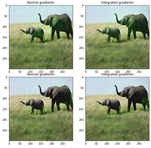
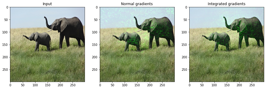
vis = GradVisualizer()
vis.visualize(
    image=orig_img,
    gradients=grads[0].numpy(),
    integrated_gradients=igrads.numpy(),
    clip_above_percentile=99,
    clip_below_percentile=0,
)

vis.visualize(
    image=orig_img,
    gradients=grads[0].numpy(),
    integrated_gradients=igrads.numpy(),
    clip_above_percentile=95,
    clip_below_percentile=28,
    morphological_cleanup=True,
    outlines=True,
)

Predicted: tf.Tensor(386, shape=(), dtype=int64) [('n02504458', 'African_elephant', 0.8871446)]

以上