Keras 2 : examples : セマンティック画像クラスタリング (翻訳/解説)
翻訳 : (株)クラスキャット セールスインフォメーション
作成日時 : 12/13/2021 (keras 2.7.0)
* 本ページは、Keras の以下のドキュメントを翻訳した上で適宜、補足説明したものです:
- Code examples : Computer Vision : Semantic Image Clustering (Author: Khalid Salama)
* サンプルコードの動作確認はしておりますが、必要な場合には適宜、追加改変しています。
* ご自由にリンクを張って頂いてかまいませんが、sales-info@classcat.com までご一報いただけると嬉しいです。

- 人工知能研究開発支援
- 人工知能研修サービス(経営者層向けオンサイト研修)
- テクニカルコンサルティングサービス
- 実証実験(プロトタイプ構築)
- アプリケーションへの実装
- 人工知能研修サービス
- PoC(概念実証)を失敗させないための支援
- お住まいの地域に関係なく Web ブラウザからご参加頂けます。事前登録 が必要ですのでご注意ください。
◆ お問合せ : 本件に関するお問い合わせ先は下記までお願いいたします。
- 株式会社クラスキャット セールス・マーケティング本部 セールス・インフォメーション
- sales-info@classcat.com ; Web: www.classcat.com ; ClassCatJP

Keras 2 : examples : セマンティック画像クラスタリング
Description: Adopting Nearest neighbors (SCAN) アルゴリズムによるセマンティック・クラスタリング。
イントロダクション
このサンプルは CIFAR-10 データセット上で Semantic Clustering by Adopting Nearest neighbors (SCAN) アルゴリズム (Van Gansbeke et al., 2020) を適用する方法を実演します。このアルゴリズムは 2 つの段階から構成されます :
- 画像の自己教師あり視覚表現学習、そこでは simCLR テクニックを使用します。
- 隣接するベクトルのクラスタ割当て間の一致 (= agreement) を最大化するために学習された視覚表現ベクトルをクラスタリングする。
このサンプルは TensorFlow Addons を必要とします、これは次のコマンドを使用してインストールできます :
pip install tensorflow-addons
セットアップ
from collections import defaultdict
import random
import numpy as np
import tensorflow as tf
import tensorflow_addons as tfa
from tensorflow import keras
from tensorflow.keras import layers
import matplotlib.pyplot as plt
from tqdm import tqdm
データの準備
num_classes = 10
input_shape = (32, 32, 3)

(x_train, y_train), (x_test, y_test) = keras.datasets.cifar10.load_data()
x_data = np.concatenate([x_train, x_test])
y_data = np.concatenate([y_train, y_test])

print("x_data shape:", x_data.shape, "- y_data shape:", y_data.shape)

classes = [
    "airplane",
    "automobile",
    "bird",
    "cat",
    "deer",
    "dog",
    "frog",
    "horse",
    "ship",
    "truck",
]
x_data shape: (60000, 32, 32, 3) - y_data shape: (60000, 1)
ハイパーパラメータの定義
target_size = 32  # Resize the input images.
representation_dim = 512  # The dimensions of the features vector.
projection_units = 128  # The projection head of the representation learner.
num_clusters = 20  # Number of clusters.
k_neighbours = 5  # Number of neighbours to consider during cluster learning.
tune_encoder_during_clustering = False  # Freeze the encoder in the cluster learning.
データ前処理の実装
データ前処理ステップは入力画像を望まれる target_size にリサイズして特徴毎に正規化を適用します。視覚エンコーダとして keras.applications.ResNet50V2 を使用するとき、画像の 255 x 255 入力へのリサイズはより正確な結果になりますがより長時間の訓練が必要となることに注意してください。
data_preprocessing = keras.Sequential(
    [
        layers.Resizing(target_size, target_size),
        layers.Normalization(),
    ]
)
# Compute the mean and the variance from the data for normalization.
data_preprocessing.layers[-1].adapt(x_data)
データ増強
入力画像に適用する単一のデータ増強関数をランダムに選択する simCLR とは違い、データ増強関数のセットを入力画像にランダムに適用します。(データ増強チュートリアル に従って他の画像増強テクニックで実験することができます。)
data_augmentation = keras.Sequential(
    [
        layers.RandomTranslation(
            height_factor=(-0.2, 0.2), width_factor=(-0.2, 0.2), fill_mode="nearest"
        ),
        layers.RandomFlip(mode="horizontal"),
        layers.RandomRotation(
            factor=0.15, fill_mode="nearest"
        ),
        layers.RandomZoom(
            height_factor=(-0.3, 0.1), width_factor=(-0.3, 0.1), fill_mode="nearest"
        )
    ]
)
ランダム画像を表示します。
image_idx = np.random.choice(range(x_data.shape[0]))
image = x_data[image_idx]
image_class = classes[y_data[image_idx][0]]
plt.figure(figsize=(3, 3))
plt.imshow(x_data[image_idx].astype("uint8"))
plt.title(image_class)
_ = plt.axis("off")

画像の増強バージョンのサンプルを表示します。
plt.figure(figsize=(10, 10))
for i in range(9):
    augmented_images = data_augmentation(np.array([image]))
    ax = plt.subplot(3, 3, i + 1)
    plt.imshow(augmented_images[0].numpy().astype("uint8"))
    plt.axis("off")


自己教師あり表現学習
視覚エンコーダの実装
def create_encoder(representation_dim):
    encoder = keras.Sequential(
        [
            keras.applications.ResNet50V2(
                include_top=False, weights=None, pooling="avg"
            ),
            layers.Dense(representation_dim),
        ]
    )
    return encoder
教師なし対照損失
class RepresentationLearner(keras.Model):
    def __init__(
        self,
        encoder,
        projection_units,
        num_augmentations,
        temperature=1.0,
        dropout_rate=0.1,
        l2_normalize=False,
        **kwargs
    ):
        super(RepresentationLearner, self).__init__(**kwargs)
        self.encoder = encoder
        # Create projection head.
        self.projector = keras.Sequential(
            [
                layers.Dropout(dropout_rate),
                layers.Dense(units=projection_units, use_bias=False),
                layers.BatchNormalization(),
                layers.ReLU(),
            ]
        )
        self.num_augmentations = num_augmentations
        self.temperature = temperature
        self.l2_normalize = l2_normalize
        self.loss_tracker = keras.metrics.Mean(name="loss")

    @property
    def metrics(self):
        return [self.loss_tracker]

    def compute_contrastive_loss(self, feature_vectors, batch_size):
        num_augmentations = tf.shape(feature_vectors)[0] // batch_size
        if self.l2_normalize:
            feature_vectors = tf.math.l2_normalize(feature_vectors, -1)
        # The logits shape is [num_augmentations * batch_size, num_augmentations * batch_size].
        logits = (
            tf.linalg.matmul(feature_vectors, feature_vectors, transpose_b=True)
            / self.temperature
        )
        # Apply log-max trick for numerical stability.
        logits_max = tf.math.reduce_max(logits, axis=1)
        logits = logits - logits_max
        # The shape of targets is [num_augmentations * batch_size, num_augmentations * batch_size].
        # targets is a matrix consits of num_augmentations submatrices of shape [batch_size * batch_size].
        # Each [batch_size * batch_size] submatrix is an identity matrix (diagonal entries are ones).
        targets = tf.tile(tf.eye(batch_size), [num_augmentations, num_augmentations])
        # Compute cross entropy loss
        return keras.losses.categorical_crossentropy(
            y_true=targets, y_pred=logits, from_logits=True
        )

    def call(self, inputs):
        # Preprocess the input images.
        preprocessed = data_preprocessing(inputs)
        # Create augmented versions of the images.
        augmented = []
        for _ in range(self.num_augmentations):
            augmented.append(data_augmentation(preprocessed))
        augmented = layers.Concatenate(axis=0)(augmented)
        # Generate embedding representations of the images.
        features = self.encoder(augmented)
        # Apply projection head.
        return self.projector(features)

    def train_step(self, inputs):
        batch_size = tf.shape(inputs)[0]
        # Run the forward pass and compute the contrastive loss
        with tf.GradientTape() as tape:
            feature_vectors = self(inputs, training=True)
            loss = self.compute_contrastive_loss(feature_vectors, batch_size)
        # Compute gradients
        trainable_vars = self.trainable_variables
        gradients = tape.gradient(loss, trainable_vars)
        # Update weights
        self.optimizer.apply_gradients(zip(gradients, trainable_vars))
        # Update loss tracker metric
        self.loss_tracker.update_state(loss)
        # Return a dict mapping metric names to current value
        return {m.name: m.result() for m in self.metrics}

    def test_step(self, inputs):
        batch_size = tf.shape(inputs)[0]
        feature_vectors = self(inputs, training=False)
        loss = self.compute_contrastive_loss(feature_vectors, batch_size)
        self.loss_tracker.update_state(loss)
        return {"loss": self.loss_tracker.result()}
モデルの訓練
# Create vision encoder.
encoder = create_encoder(representation_dim)
# Create representation learner.
representation_learner = RepresentationLearner(
    encoder, projection_units, num_augmentations=2, temperature=0.1
)
# Create a a Cosine decay learning rate scheduler.
lr_scheduler = keras.optimizers.schedules.CosineDecay(
    initial_learning_rate=0.001, decay_steps=500, alpha=0.1
)
# Compile the model.
representation_learner.compile(
    optimizer=tfa.optimizers.AdamW(learning_rate=lr_scheduler, weight_decay=0.0001),
)
# Fit the model.
history = representation_learner.fit(
    x=x_data,
    batch_size=512,
    epochs=50,  # for better results, increase the number of epochs to 500.
)
Epoch 1/50
118/118 [==============================] - 29s 135ms/step - loss: 41.1135
Epoch 2/50
118/118 [==============================] - 15s 125ms/step - loss: 11.7141
Epoch 3/50
118/118 [==============================] - 15s 125ms/step - loss: 11.1728
Epoch 4/50
118/118 [==============================] - 15s 125ms/step - loss: 10.9717
Epoch 5/50
118/118 [==============================] - 15s 125ms/step - loss: 10.8574
Epoch 6/50
118/118 [==============================] - 15s 125ms/step - loss: 10.9496
Epoch 7/50
118/118 [==============================] - 15s 124ms/step - loss: 10.7493
Epoch 8/50
118/118 [==============================] - 15s 124ms/step - loss: 10.5979
Epoch 9/50
118/118 [==============================] - 15s 124ms/step - loss: 10.4613
Epoch 10/50
118/118 [==============================] - 15s 125ms/step - loss: 10.2900
Epoch 11/50
118/118 [==============================] - 15s 124ms/step - loss: 10.1303
Epoch 12/50
118/118 [==============================] - 15s 124ms/step - loss: 9.9608
Epoch 13/50
118/118 [==============================] - 15s 124ms/step - loss: 9.7788
Epoch 14/50
118/118 [==============================] - 15s 124ms/step - loss: 9.5830
Epoch 15/50
118/118 [==============================] - 15s 124ms/step - loss: 9.4038
Epoch 16/50
118/118 [==============================] - 15s 124ms/step - loss: 9.1887
Epoch 17/50
118/118 [==============================] - 15s 124ms/step - loss: 9.0000
Epoch 18/50
118/118 [==============================] - 15s 124ms/step - loss: 8.7764
Epoch 19/50
118/118 [==============================] - 15s 124ms/step - loss: 8.5784
Epoch 20/50
118/118 [==============================] - 15s 124ms/step - loss: 8.3592
Epoch 21/50
118/118 [==============================] - 15s 124ms/step - loss: 8.2545
Epoch 22/50
118/118 [==============================] - 15s 124ms/step - loss: 8.1171
Epoch 23/50
118/118 [==============================] - 15s 124ms/step - loss: 7.9598
Epoch 24/50
118/118 [==============================] - 15s 124ms/step - loss: 7.8623
Epoch 25/50
118/118 [==============================] - 15s 124ms/step - loss: 7.7169
Epoch 26/50
118/118 [==============================] - 15s 124ms/step - loss: 7.5100
Epoch 27/50
118/118 [==============================] - 15s 124ms/step - loss: 7.5887
Epoch 28/50
118/118 [==============================] - 15s 124ms/step - loss: 7.3511
Epoch 29/50
118/118 [==============================] - 15s 124ms/step - loss: 7.1647
Epoch 30/50
118/118 [==============================] - 15s 124ms/step - loss: 7.1549
Epoch 31/50
118/118 [==============================] - 15s 124ms/step - loss: 7.0462
Epoch 32/50
118/118 [==============================] - 15s 124ms/step - loss: 6.8149
Epoch 33/50
118/118 [==============================] - 15s 124ms/step - loss: 6.6954
Epoch 34/50
118/118 [==============================] - 15s 124ms/step - loss: 6.5354
Epoch 35/50
118/118 [==============================] - 15s 124ms/step - loss: 6.3982
Epoch 36/50
118/118 [==============================] - 15s 124ms/step - loss: 6.4175
Epoch 37/50
118/118 [==============================] - 15s 124ms/step - loss: 6.3820
Epoch 38/50
118/118 [==============================] - 15s 124ms/step - loss: 6.2560
Epoch 39/50
118/118 [==============================] - 15s 124ms/step - loss: 6.1237
Epoch 40/50
118/118 [==============================] - 15s 124ms/step - loss: 6.0485
Epoch 41/50
118/118 [==============================] - 15s 124ms/step - loss: 5.8846
Epoch 42/50
118/118 [==============================] - 15s 124ms/step - loss: 5.7548
Epoch 43/50
118/118 [==============================] - 15s 124ms/step - loss: 6.0794
Epoch 44/50
118/118 [==============================] - 15s 124ms/step - loss: 5.9023
Epoch 45/50
118/118 [==============================] - 15s 124ms/step - loss: 5.9548
Epoch 46/50
118/118 [==============================] - 15s 124ms/step - loss: 6.0809
Epoch 47/50
118/118 [==============================] - 15s 124ms/step - loss: 5.6123
Epoch 48/50
118/118 [==============================] - 15s 124ms/step - loss: 5.5667
Epoch 49/50
118/118 [==============================] - 15s 124ms/step - loss: 5.4573
Epoch 50/50
118/118 [==============================] - 15s 124ms/step - loss: 5.4597
(訳者注: 実験結果)
Epoch 1/50
118/118 [==============================] - 29s 87ms/step - loss: 29.9556
Epoch 2/50
118/118 [==============================] - 9s 77ms/step - loss: 11.5125
Epoch 3/50
118/118 [==============================] - 9s 78ms/step - loss: 11.0072
Epoch 4/50
118/118 [==============================] - 9s 78ms/step - loss: 10.7874
Epoch 5/50
118/118 [==============================] - 9s 78ms/step - loss: 10.6437
Epoch 6/50
118/118 [==============================] - 9s 78ms/step - loss: 10.5506
Epoch 7/50
118/118 [==============================] - 9s 78ms/step - loss: 10.4373
Epoch 8/50
118/118 [==============================] - 9s 78ms/step - loss: 10.2851
Epoch 9/50
118/118 [==============================] - 9s 78ms/step - loss: 10.1732
Epoch 10/50
118/118 [==============================] - 9s 78ms/step - loss: 9.9649
Epoch 11/50
118/118 [==============================] - 9s 77ms/step - loss: 9.8258
Epoch 12/50
118/118 [==============================] - 9s 78ms/step - loss: 9.5910
Epoch 13/50
118/118 [==============================] - 9s 78ms/step - loss: 9.3802
Epoch 14/50
118/118 [==============================] - 9s 78ms/step - loss: 9.1439
Epoch 15/50
118/118 [==============================] - 9s 78ms/step - loss: 8.9558
Epoch 16/50
118/118 [==============================] - 9s 78ms/step - loss: 8.7526
Epoch 17/50
118/118 [==============================] - 9s 78ms/step - loss: 8.6240
Epoch 18/50
118/118 [==============================] - 9s 78ms/step - loss: 8.4214
Epoch 19/50
118/118 [==============================] - 9s 78ms/step - loss: 8.2466
Epoch 20/50
118/118 [==============================] - 9s 78ms/step - loss: 8.1365
Epoch 21/50
118/118 [==============================] - 9s 77ms/step - loss: 7.9626
Epoch 22/50
118/118 [==============================] - 9s 78ms/step - loss: 7.9407
Epoch 23/50
118/118 [==============================] - 9s 78ms/step - loss: 7.7123
Epoch 24/50
118/118 [==============================] - 9s 78ms/step - loss: 7.6336
Epoch 25/50
118/118 [==============================] - 9s 77ms/step - loss: 7.4061
Epoch 26/50
118/118 [==============================] - 9s 77ms/step - loss: 7.3237
Epoch 27/50
118/118 [==============================] - 9s 77ms/step - loss: 7.1124
Epoch 28/50
118/118 [==============================] - 9s 78ms/step - loss: 6.9913
Epoch 29/50
118/118 [==============================] - 9s 78ms/step - loss: 6.8683
Epoch 30/50
118/118 [==============================] - 9s 78ms/step - loss: 7.0046
Epoch 31/50
118/118 [==============================] - 9s 78ms/step - loss: 6.6838
Epoch 32/50
118/118 [==============================] - 9s 78ms/step - loss: 6.5952
Epoch 33/50
118/118 [==============================] - 9s 78ms/step - loss: 6.4429
Epoch 34/50
118/118 [==============================] - 9s 78ms/step - loss: 6.8122
Epoch 35/50
118/118 [==============================] - 9s 78ms/step - loss: 6.4525
Epoch 36/50
118/118 [==============================] - 9s 78ms/step - loss: 6.3212
Epoch 37/50
118/118 [==============================] - 9s 78ms/step - loss: 6.5632
Epoch 38/50
118/118 [==============================] - 9s 78ms/step - loss: 6.1890
Epoch 39/50
118/118 [==============================] - 9s 77ms/step - loss: 5.9394
Epoch 40/50
118/118 [==============================] - 9s 78ms/step - loss: 5.8260
Epoch 41/50
118/118 [==============================] - 9s 77ms/step - loss: 5.6711
Epoch 42/50
118/118 [==============================] - 9s 78ms/step - loss: 5.7763
Epoch 43/50
118/118 [==============================] - 9s 78ms/step - loss: 5.8551
Epoch 44/50
118/118 [==============================] - 9s 78ms/step - loss: 5.7423
Epoch 45/50
118/118 [==============================] - 9s 78ms/step - loss: 5.9383
Epoch 46/50
118/118 [==============================] - 9s 78ms/step - loss: 5.5107
Epoch 47/50
118/118 [==============================] - 9s 78ms/step - loss: 5.7404
Epoch 48/50
118/118 [==============================] - 9s 78ms/step - loss: 5.3652
Epoch 49/50
118/118 [==============================] - 9s 78ms/step - loss: 5.2598
Epoch 50/50
118/118 [==============================] - 9s 78ms/step - loss: 5.2350
CPU times: user 9min 3s, sys: 30.9 s, total: 9min 34s
Wall time: 8min
訓練損失のプロット
plt.plot(history.history["loss"])
plt.ylabel("loss")
plt.xlabel("epoch")
plt.show()


最近傍の計算
画像に対する埋め込みの生成
batch_size = 500
# Get the feature vector representations of the images.
feature_vectors = encoder.predict(x_data, batch_size=batch_size, verbose=1)
# Normalize the feature vectores.
feature_vectors = tf.math.l2_normalize(feature_vectors, -1)
120/120 [==============================] - 4s 18ms/step
各埋め込みに対する k 近傍を見つける
neighbours = []
num_batches = feature_vectors.shape[0] // batch_size
for batch_idx in tqdm(range(num_batches)):
    start_idx = batch_idx * batch_size
    end_idx = start_idx + batch_size
    current_batch = feature_vectors[start_idx:end_idx]
    # Compute the dot similarity.
    similarities = tf.linalg.matmul(current_batch, feature_vectors, transpose_b=True)
    # Get the indices of most similar vectors.
    _, indices = tf.math.top_k(similarities, k=k_neighbours + 1, sorted=True)
    # Add the indices to the neighbours.
    neighbours.append(indices[..., 1:])

neighbours = np.reshape(np.array(neighbours), (-1, k_neighbours))
各行で幾つかの近傍を表示しましょう :
nrows = 4
ncols = k_neighbours + 1

plt.figure(figsize=(12, 12))
position = 1
for _ in range(nrows):
    anchor_idx = np.random.choice(range(x_data.shape[0]))
    neighbour_indicies = neighbours[anchor_idx]
    indices = [anchor_idx] + neighbour_indicies.tolist()
    for j in range(ncols):
        plt.subplot(nrows, ncols, position)
        plt.imshow(x_data[indices[j]].astype("uint8"))
        plt.title(classes[y_data[indices[j]][0]])
        plt.axis("off")
        position += 1

各行の画像が視覚的に似ていて、類似のクラスに属していることに気付くでしょう。
近傍によるセマンティック・クラスタリング
クラスタリング一貫性損失の実装
この損失は近傍が同じクラスタリング割当てを持つことを確実にしようとします。
class ClustersConsistencyLoss(keras.losses.Loss):
    def __init__(self):
        super(ClustersConsistencyLoss, self).__init__()

    def __call__(self, target, similarity, sample_weight=None):
        # Set targets to be ones.
        target = tf.ones_like(similarity)
        # Compute cross entropy loss.
        loss = keras.losses.binary_crossentropy(
            y_true=target, y_pred=similarity, from_logits=True
        )
        return tf.math.reduce_mean(loss)
クラスタ・エントロピー損失の実装
この損失は、インスタンスの殆どが一つのクラスに割当てられることを回避するため、クラスタ分布がおおよそ一様であることを確実にしようとします。
class ClustersEntropyLoss(keras.losses.Loss):
    def __init__(self, entropy_loss_weight=1.0):
        super(ClustersEntropyLoss, self).__init__()
        self.entropy_loss_weight = entropy_loss_weight

    def __call__(self, target, cluster_probabilities, sample_weight=None):
        # Ideal entropy = log(num_clusters).
        num_clusters = tf.cast(tf.shape(cluster_probabilities)[-1], tf.dtypes.float32)
        target = tf.math.log(num_clusters)
        # Compute the overall clusters distribution.
        cluster_probabilities = tf.math.reduce_mean(cluster_probabilities, axis=0)
        # Replacing zero probabilities - if any - with a very small value.
        cluster_probabilities = tf.clip_by_value(
            cluster_probabilities, clip_value_min=1e-8, clip_value_max=1.0
        )
        # Compute the entropy over the clusters.
        entropy = -tf.math.reduce_sum(
            cluster_probabilities * tf.math.log(cluster_probabilities)
        )
        # Compute the difference between the target and the actual.
        loss = target - entropy
        return loss
クラスタリング・モデルの実装
このモデルは入力として raw 画像を取り、訓練済みのエンコーダを使用してその特徴ベクトルを生成し、そしてクラスタ割当てとして特徴ベクトルを与えて、クラスタの確率分布を生成します。
def create_clustering_model(encoder, num_clusters, name=None):
    inputs = keras.Input(shape=input_shape)
    # Preprocess the input images.
    preprocessed = data_preprocessing(inputs)
    # Apply data augmentation to the images.
    augmented = data_augmentation(preprocessed)
    # Generate embedding representations of the images.
    features = encoder(augmented)
    # Assign the images to clusters.
    outputs = layers.Dense(units=num_clusters, activation="softmax")(features)
    # Create the model.
    model = keras.Model(inputs=inputs, outputs=outputs, name=name)
    return model
クラスタリング学習器 (= learner) の実装
このモデルは入力アンカー画像とその近傍を受け取り、clustering_model モデルを使用してそれらのためのクラスタ割当てを生成し、2 つの出力を生成します :
- similarity : アンカー画像とその近傍のクラスタ割当て間の類似度。この出力は ClustersConsistencyLoss に供給されます。
- anchor_clustering : アンカー画像のクラスタ割当て。これは ClustersEntropyLoss に供給されます。
def create_clustering_learner(clustering_model):
    anchor = keras.Input(shape=input_shape, name="anchors")
    neighbours = keras.Input(
        shape=tuple([k_neighbours]) + input_shape, name="neighbours"
    )
    # Changes neighbours shape to [batch_size * k_neighbours, width, height, channels]
    neighbours_reshaped = tf.reshape(neighbours, shape=tuple([-1]) + input_shape)
    # anchor_clustering shape: [batch_size, num_clusters]
    anchor_clustering = clustering_model(anchor)
    # neighbours_clustering shape: [batch_size * k_neighbours, num_clusters]
    neighbours_clustering = clustering_model(neighbours_reshaped)
    # Convert neighbours_clustering shape to [batch_size, k_neighbours, num_clusters]
    neighbours_clustering = tf.reshape(
        neighbours_clustering,
        shape=(-1, k_neighbours, tf.shape(neighbours_clustering)[-1]),
    )
    # similarity shape: [batch_size, 1, k_neighbours]
    similarity = tf.linalg.einsum(
        "bij,bkj->bik", tf.expand_dims(anchor_clustering, axis=1), neighbours_clustering
    )
    # similarity shape:  [batch_size, k_neighbours]
    similarity = layers.Lambda(lambda x: tf.squeeze(x, axis=1), name="similarity")(
        similarity
    )
    # Create the model.
    model = keras.Model(
        inputs=[anchor, neighbours],
        outputs=[similarity, anchor_clustering],
        name="clustering_learner",
    )
    return model
モデルの訓練
# If tune_encoder_during_clustering is set to False,
# then freeze the encoder weights.
for layer in encoder.layers:
    layer.trainable = tune_encoder_during_clustering
# Create the clustering model and learner.
clustering_model = create_clustering_model(encoder, num_clusters, name="clustering")
clustering_learner = create_clustering_learner(clustering_model)
# Instantiate the model losses.
losses = [ClustersConsistencyLoss(), ClustersEntropyLoss(entropy_loss_weight=5)]
# Create the model inputs and labels.
inputs = {"anchors": x_data, "neighbours": tf.gather(x_data, neighbours)}
labels = tf.ones(shape=(x_data.shape[0]))
# Compile the model.
clustering_learner.compile(
    optimizer=tfa.optimizers.AdamW(learning_rate=0.0005, weight_decay=0.0001),
    loss=losses,
)

# Begin training the model.
clustering_learner.fit(x=inputs, y=labels, batch_size=512, epochs=50)
Epoch 1/50
118/118 [==============================] - 20s 95ms/step - loss: 0.6655 - similarity_loss: 0.6642 - clustering_loss: 0.0013
Epoch 2/50
118/118 [==============================] - 10s 86ms/step - loss: 0.6361 - similarity_loss: 0.6325 - clustering_loss: 0.0036
Epoch 3/50
118/118 [==============================] - 10s 85ms/step - loss: 0.6129 - similarity_loss: 0.6070 - clustering_loss: 0.0059
Epoch 4/50
118/118 [==============================] - 10s 85ms/step - loss: 0.6005 - similarity_loss: 0.5930 - clustering_loss: 0.0075
Epoch 5/50
118/118 [==============================] - 10s 85ms/step - loss: 0.5923 - similarity_loss: 0.5849 - clustering_loss: 0.0074
Epoch 6/50
118/118 [==============================] - 10s 86ms/step - loss: 0.5879 - similarity_loss: 0.5795 - clustering_loss: 0.0084
Epoch 7/50
118/118 [==============================] - 10s 85ms/step - loss: 0.5841 - similarity_loss: 0.5754 - clustering_loss: 0.0087
Epoch 8/50
118/118 [==============================] - 10s 85ms/step - loss: 0.5817 - similarity_loss: 0.5733 - clustering_loss: 0.0084
Epoch 9/50
118/118 [==============================] - 10s 85ms/step - loss: 0.5811 - similarity_loss: 0.5717 - clustering_loss: 0.0094
Epoch 10/50
118/118 [==============================] - 10s 85ms/step - loss: 0.5797 - similarity_loss: 0.5697 - clustering_loss: 0.0100
Epoch 11/50
118/118 [==============================] - 10s 86ms/step - loss: 0.5767 - similarity_loss: 0.5676 - clustering_loss: 0.0091
Epoch 12/50
118/118 [==============================] - 10s 86ms/step - loss: 0.5771 - similarity_loss: 0.5667 - clustering_loss: 0.0104
Epoch 13/50
118/118 [==============================] - 10s 86ms/step - loss: 0.5755 - similarity_loss: 0.5661 - clustering_loss: 0.0094
Epoch 14/50
118/118 [==============================] - 10s 86ms/step - loss: 0.5746 - similarity_loss: 0.5653 - clustering_loss: 0.0093
Epoch 15/50
118/118 [==============================] - 10s 86ms/step - loss: 0.5743 - similarity_loss: 0.5640 - clustering_loss: 0.0103
Epoch 16/50
118/118 [==============================] - 10s 86ms/step - loss: 0.5738 - similarity_loss: 0.5636 - clustering_loss: 0.0102
Epoch 17/50
118/118 [==============================] - 10s 86ms/step - loss: 0.5732 - similarity_loss: 0.5627 - clustering_loss: 0.0106
Epoch 18/50
118/118 [==============================] - 10s 86ms/step - loss: 0.5723 - similarity_loss: 0.5621 - clustering_loss: 0.0102
Epoch 19/50
118/118 [==============================] - 10s 86ms/step - loss: 0.5711 - similarity_loss: 0.5615 - clustering_loss: 0.0096
Epoch 20/50
118/118 [==============================] - 10s 86ms/step - loss: 0.5693 - similarity_loss: 0.5596 - clustering_loss: 0.0097
Epoch 21/50
118/118 [==============================] - 10s 86ms/step - loss: 0.5699 - similarity_loss: 0.5600 - clustering_loss: 0.0099
Epoch 22/50
118/118 [==============================] - 10s 86ms/step - loss: 0.5694 - similarity_loss: 0.5592 - clustering_loss: 0.0102
Epoch 23/50
118/118 [==============================] - 10s 86ms/step - loss: 0.5703 - similarity_loss: 0.5595 - clustering_loss: 0.0108
Epoch 24/50
118/118 [==============================] - 10s 86ms/step - loss: 0.5687 - similarity_loss: 0.5587 - clustering_loss: 0.0101
Epoch 25/50
118/118 [==============================] - 10s 86ms/step - loss: 0.5688 - similarity_loss: 0.5585 - clustering_loss: 0.0103
Epoch 26/50
118/118 [==============================] - 10s 86ms/step - loss: 0.5690 - similarity_loss: 0.5583 - clustering_loss: 0.0108
Epoch 27/50
118/118 [==============================] - 10s 86ms/step - loss: 0.5679 - similarity_loss: 0.5572 - clustering_loss: 0.0107
Epoch 28/50
118/118 [==============================] - 10s 86ms/step - loss: 0.5681 - similarity_loss: 0.5573 - clustering_loss: 0.0108
Epoch 29/50
118/118 [==============================] - 10s 86ms/step - loss: 0.5682 - similarity_loss: 0.5572 - clustering_loss: 0.0111
Epoch 30/50
118/118 [==============================] - 10s 86ms/step - loss: 0.5675 - similarity_loss: 0.5571 - clustering_loss: 0.0104
Epoch 31/50
118/118 [==============================] - 10s 86ms/step - loss: 0.5679 - similarity_loss: 0.5562 - clustering_loss: 0.0116
Epoch 32/50
118/118 [==============================] - 10s 86ms/step - loss: 0.5663 - similarity_loss: 0.5554 - clustering_loss: 0.0109
Epoch 33/50
118/118 [==============================] - 10s 86ms/step - loss: 0.5665 - similarity_loss: 0.5556 - clustering_loss: 0.0109
Epoch 34/50
118/118 [==============================] - 10s 86ms/step - loss: 0.5679 - similarity_loss: 0.5568 - clustering_loss: 0.0111
Epoch 35/50
118/118 [==============================] - 10s 86ms/step - loss: 0.5680 - similarity_loss: 0.5563 - clustering_loss: 0.0117
Epoch 36/50
118/118 [==============================] - 10s 86ms/step - loss: 0.5665 - similarity_loss: 0.5553 - clustering_loss: 0.0112
Epoch 37/50
118/118 [==============================] - 10s 86ms/step - loss: 0.5674 - similarity_loss: 0.5556 - clustering_loss: 0.0118
Epoch 38/50
118/118 [==============================] - 10s 86ms/step - loss: 0.5648 - similarity_loss: 0.5543 - clustering_loss: 0.0105
Epoch 39/50
118/118 [==============================] - 10s 86ms/step - loss: 0.5653 - similarity_loss: 0.5549 - clustering_loss: 0.0103
Epoch 40/50
118/118 [==============================] - 10s 86ms/step - loss: 0.5656 - similarity_loss: 0.5544 - clustering_loss: 0.0113
Epoch 41/50
118/118 [==============================] - 10s 86ms/step - loss: 0.5644 - similarity_loss: 0.5542 - clustering_loss: 0.0102
Epoch 42/50
118/118 [==============================] - 10s 86ms/step - loss: 0.5658 - similarity_loss: 0.5540 - clustering_loss: 0.0118
Epoch 43/50
118/118 [==============================] - 10s 86ms/step - loss: 0.5655 - similarity_loss: 0.5539 - clustering_loss: 0.0116
Epoch 44/50
118/118 [==============================] - 10s 87ms/step - loss: 0.5662 - similarity_loss: 0.5543 - clustering_loss: 0.0119
Epoch 45/50
118/118 [==============================] - 10s 86ms/step - loss: 0.5651 - similarity_loss: 0.5537 - clustering_loss: 0.0114
Epoch 46/50
118/118 [==============================] - 10s 86ms/step - loss: 0.5635 - similarity_loss: 0.5534 - clustering_loss: 0.0101
Epoch 47/50
118/118 [==============================] - 10s 86ms/step - loss: 0.5633 - similarity_loss: 0.5529 - clustering_loss: 0.0103
Epoch 48/50
118/118 [==============================] - 10s 86ms/step - loss: 0.5643 - similarity_loss: 0.5526 - clustering_loss: 0.0117
Epoch 49/50
118/118 [==============================] - 10s 86ms/step - loss: 0.5653 - similarity_loss: 0.5532 - clustering_loss: 0.0121
Epoch 50/50
118/118 [==============================] - 10s 86ms/step - loss: 0.5641 - similarity_loss: 0.5525 - clustering_loss: 0.0117

<tensorflow.python.keras.callbacks.History at 0x7f1da373ea10>
Epoch 1/50
118/118 [==============================] - 16s 70ms/step - loss: 0.6686 - similarity_loss: 0.6683 - clustering_loss: 3.3759e-04
Epoch 2/50
118/118 [==============================] - 7s 63ms/step - loss: 0.6681 - similarity_loss: 0.6679 - clustering_loss: 2.2749e-04
Epoch 3/50
118/118 [==============================] - 7s 63ms/step - loss: 0.6674 - similarity_loss: 0.6670 - clustering_loss: 4.8134e-04
Epoch 4/50
118/118 [==============================] - 7s 63ms/step - loss: 0.6668 - similarity_loss: 0.6660 - clustering_loss: 7.9841e-04
Epoch 5/50
118/118 [==============================] - 7s 63ms/step - loss: 0.6659 - similarity_loss: 0.6651 - clustering_loss: 8.5452e-04
Epoch 6/50
118/118 [==============================] - 7s 63ms/step - loss: 0.6656 - similarity_loss: 0.6644 - clustering_loss: 0.0012
Epoch 7/50
118/118 [==============================] - 7s 63ms/step - loss: 0.6651 - similarity_loss: 0.6637 - clustering_loss: 0.0014
Epoch 8/50
118/118 [==============================] - 7s 63ms/step - loss: 0.6649 - similarity_loss: 0.6633 - clustering_loss: 0.0016
Epoch 9/50
118/118 [==============================] - 7s 63ms/step - loss: 0.6647 - similarity_loss: 0.6629 - clustering_loss: 0.0017
Epoch 10/50
118/118 [==============================] - 7s 63ms/step - loss: 0.6641 - similarity_loss: 0.6626 - clustering_loss: 0.0015
Epoch 11/50
118/118 [==============================] - 7s 63ms/step - loss: 0.6641 - similarity_loss: 0.6623 - clustering_loss: 0.0018
Epoch 12/50
118/118 [==============================] - 7s 63ms/step - loss: 0.6638 - similarity_loss: 0.6619 - clustering_loss: 0.0018
Epoch 13/50
118/118 [==============================] - 7s 63ms/step - loss: 0.6636 - similarity_loss: 0.6617 - clustering_loss: 0.0019
Epoch 14/50
118/118 [==============================] - 7s 63ms/step - loss: 0.6635 - similarity_loss: 0.6615 - clustering_loss: 0.0020
Epoch 15/50
118/118 [==============================] - 7s 63ms/step - loss: 0.6633 - similarity_loss: 0.6613 - clustering_loss: 0.0020
Epoch 16/50
118/118 [==============================] - 7s 63ms/step - loss: 0.6632 - similarity_loss: 0.6612 - clustering_loss: 0.0020
Epoch 17/50
118/118 [==============================] - 7s 63ms/step - loss: 0.6634 - similarity_loss: 0.6609 - clustering_loss: 0.0025
Epoch 18/50
118/118 [==============================] - 7s 63ms/step - loss: 0.6630 - similarity_loss: 0.6608 - clustering_loss: 0.0022
Epoch 19/50
118/118 [==============================] - 7s 63ms/step - loss: 0.6633 - similarity_loss: 0.6607 - clustering_loss: 0.0026
Epoch 20/50
118/118 [==============================] - 7s 63ms/step - loss: 0.6632 - similarity_loss: 0.6606 - clustering_loss: 0.0026
Epoch 21/50
118/118 [==============================] - 7s 63ms/step - loss: 0.6628 - similarity_loss: 0.6605 - clustering_loss: 0.0023
Epoch 22/50
118/118 [==============================] - 7s 63ms/step - loss: 0.6628 - similarity_loss: 0.6603 - clustering_loss: 0.0025
Epoch 23/50
118/118 [==============================] - 7s 63ms/step - loss: 0.6630 - similarity_loss: 0.6603 - clustering_loss: 0.0027
Epoch 24/50
118/118 [==============================] - 7s 63ms/step - loss: 0.6626 - similarity_loss: 0.6602 - clustering_loss: 0.0024
Epoch 25/50
118/118 [==============================] - 7s 63ms/step - loss: 0.6626 - similarity_loss: 0.6601 - clustering_loss: 0.0025
Epoch 26/50
118/118 [==============================] - 7s 63ms/step - loss: 0.6627 - similarity_loss: 0.6600 - clustering_loss: 0.0027
Epoch 27/50
118/118 [==============================] - 7s 63ms/step - loss: 0.6626 - similarity_loss: 0.6600 - clustering_loss: 0.0026
Epoch 28/50
118/118 [==============================] - 7s 63ms/step - loss: 0.6627 - similarity_loss: 0.6599 - clustering_loss: 0.0028
Epoch 29/50
118/118 [==============================] - 7s 63ms/step - loss: 0.6623 - similarity_loss: 0.6599 - clustering_loss: 0.0025
Epoch 30/50
118/118 [==============================] - 7s 63ms/step - loss: 0.6623 - similarity_loss: 0.6597 - clustering_loss: 0.0026
Epoch 31/50
118/118 [==============================] - 7s 63ms/step - loss: 0.6622 - similarity_loss: 0.6597 - clustering_loss: 0.0025
Epoch 32/50
118/118 [==============================] - 7s 63ms/step - loss: 0.6623 - similarity_loss: 0.6597 - clustering_loss: 0.0026
Epoch 33/50
118/118 [==============================] - 7s 63ms/step - loss: 0.6624 - similarity_loss: 0.6596 - clustering_loss: 0.0029
Epoch 34/50
118/118 [==============================] - 7s 63ms/step - loss: 0.6626 - similarity_loss: 0.6596 - clustering_loss: 0.0031
Epoch 35/50
118/118 [==============================] - 7s 63ms/step - loss: 0.6622 - similarity_loss: 0.6595 - clustering_loss: 0.0027
Epoch 36/50
118/118 [==============================] - 7s 63ms/step - loss: 0.6622 - similarity_loss: 0.6594 - clustering_loss: 0.0028
Epoch 37/50
118/118 [==============================] - 7s 63ms/step - loss: 0.6622 - similarity_loss: 0.6594 - clustering_loss: 0.0029
Epoch 38/50
118/118 [==============================] - 7s 63ms/step - loss: 0.6623 - similarity_loss: 0.6594 - clustering_loss: 0.0029
Epoch 39/50
118/118 [==============================] - 7s 63ms/step - loss: 0.6623 - similarity_loss: 0.6594 - clustering_loss: 0.0029
Epoch 40/50
118/118 [==============================] - 7s 63ms/step - loss: 0.6623 - similarity_loss: 0.6594 - clustering_loss: 0.0029
Epoch 41/50
118/118 [==============================] - 7s 63ms/step - loss: 0.6620 - similarity_loss: 0.6593 - clustering_loss: 0.0027
Epoch 42/50
118/118 [==============================] - 7s 63ms/step - loss: 0.6621 - similarity_loss: 0.6593 - clustering_loss: 0.0028
Epoch 43/50
118/118 [==============================] - 7s 63ms/step - loss: 0.6620 - similarity_loss: 0.6593 - clustering_loss: 0.0028
Epoch 44/50
118/118 [==============================] - 7s 63ms/step - loss: 0.6621 - similarity_loss: 0.6592 - clustering_loss: 0.0029
Epoch 45/50
118/118 [==============================] - 7s 63ms/step - loss: 0.6621 - similarity_loss: 0.6592 - clustering_loss: 0.0029
Epoch 46/50
118/118 [==============================] - 7s 63ms/step - loss: 0.6621 - similarity_loss: 0.6592 - clustering_loss: 0.0029
Epoch 47/50
118/118 [==============================] - 7s 63ms/step - loss: 0.6619 - similarity_loss: 0.6591 - clustering_loss: 0.0028
Epoch 48/50
118/118 [==============================] - 7s 63ms/step - loss: 0.6624 - similarity_loss: 0.6592 - clustering_loss: 0.0032
Epoch 49/50
118/118 [==============================] - 7s 63ms/step - loss: 0.6621 - similarity_loss: 0.6591 - clustering_loss: 0.0030
Epoch 50/50
118/118 [==============================] - 7s 63ms/step - loss: 0.6621 - similarity_loss: 0.6591 - clustering_loss: 0.0030
CPU times: user 7min 18s, sys: 19.6 s, total: 7min 37s
Wall time: 6min 23s
訓練損失のプロット
plt.plot(history.history["loss"])
plt.ylabel("loss")
plt.xlabel("epoch")
plt.show()


クラスタ分析
画像のクラスタへの割当て
# Get the cluster probability distribution of the input images.
clustering_probs = clustering_model.predict(x_data, batch_size=batch_size, verbose=1)
# Get the cluster of the highest probability.
cluster_assignments = tf.math.argmax(clustering_probs, axis=-1).numpy()
# Store the clustering confidence.
# Images with the highest clustering confidence are considered the 'prototypes'
# of the clusters.
cluster_confidence = tf.math.reduce_max(clustering_probs, axis=-1).numpy()
クラスタのサイズを計算しましょう。
clusters = defaultdict(list)
for idx, c in enumerate(cluster_assignments):
    clusters[c].append((idx, cluster_confidence[idx]))

for c in range(num_clusters):
    print("cluster", c, ":", len(clusters[c]))
cluster 0 : 4132
cluster 1 : 4057
cluster 2 : 1713
cluster 3 : 2801
cluster 4 : 2511
cluster 5 : 2655
cluster 6 : 2517
cluster 7 : 4493
cluster 8 : 3687
cluster 9 : 1716
cluster 10 : 3397
cluster 11 : 3606
cluster 12 : 3325
cluster 13 : 4010
cluster 14 : 2188
cluster 15 : 3278
cluster 16 : 1902
cluster 17 : 1858
cluster 18 : 3828
cluster 19 : 2326
cluster 0 : 5102
cluster 1 : 3477
cluster 2 : 1382
cluster 3 : 5087
cluster 4 : 2589
cluster 5 : 1893
cluster 6 : 2010
cluster 7 : 5885
cluster 8 : 3072
cluster 9 : 1013
cluster 10 : 2860
cluster 11 : 4134
cluster 12 : 5173
cluster 13 : 2267
cluster 14 : 2237
cluster 15 : 2864
cluster 16 : 1281
cluster 17 : 1335
cluster 18 : 3970
cluster 19 : 2369
クラスタがおおよそ均衡の取れたサイズを持つことに気付くでしょう。
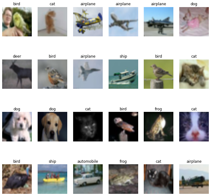
クラスタ画像の可視化
各クラスタのプロトタイプ — 最も高いクラスタリング信頼度を持つインスタンスを表示します。
num_images = 8
plt.figure(figsize=(15, 15))
position = 1
for c in range(num_clusters):
    cluster_instances = sorted(clusters[c], key=lambda kv: kv[1], reverse=True)

    for j in range(num_images):
        image_idx = cluster_instances[j][0]
        plt.subplot(num_clusters, num_images, position)
        plt.imshow(x_data[image_idx].astype("uint8"))
        plt.title(classes[y_data[image_idx][0]])
        plt.axis("off")
        position += 1

クラスタリング精度を計算する
最初に、各クラスタに対してその画像の大多数のラベルに基づいてラベルを割当てます。それから、大多数のラベルを持つ画像の数をクラスタのサイズで除算して各クラスタの精度を計算します。
cluster_label_counts = dict()

for c in range(num_clusters):
    cluster_label_counts[c] = [0] * num_classes
    instances = clusters[c]
    for i, _ in instances:
        cluster_label_counts[c][y_data[i][0]] += 1

    cluster_label_idx = np.argmax(cluster_label_counts[c])
    correct_count = np.max(cluster_label_counts[c])
    cluster_size = len(clusters[c])
    accuracy = (
        np.round((correct_count / cluster_size) * 100, 2) if cluster_size > 0 else 0
    )
    cluster_label = classes[cluster_label_idx]
    print("cluster", c, "label is:", cluster_label, " -  accuracy:", accuracy, "%")
cluster 0 label is: frog  -  accuracy: 23.11 %
cluster 1 label is: truck  -  accuracy: 23.56 %
cluster 2 label is: bird  -  accuracy: 29.01 %
cluster 3 label is: dog  -  accuracy: 16.67 %
cluster 4 label is: truck  -  accuracy: 27.8 %
cluster 5 label is: ship  -  accuracy: 36.91 %
cluster 6 label is: deer  -  accuracy: 27.89 %
cluster 7 label is: dog  -  accuracy: 23.84 %
cluster 8 label is: airplane  -  accuracy: 21.7 %
cluster 9 label is: bird  -  accuracy: 22.38 %
cluster 10 label is: automobile  -  accuracy: 24.76 %
cluster 11 label is: automobile  -  accuracy: 24.15 %
cluster 12 label is: cat  -  accuracy: 17.44 %
cluster 13 label is: truck  -  accuracy: 23.44 %
cluster 14 label is: ship  -  accuracy: 31.67 %
cluster 15 label is: airplane  -  accuracy: 41.06 %
cluster 16 label is: deer  -  accuracy: 22.77 %
cluster 17 label is: airplane  -  accuracy: 15.18 %
cluster 18 label is: frog  -  accuracy: 33.31 %
cluster 19 label is: deer  -  accuracy: 18.7 %
cluster 0 label is: truck  -  accuracy: 24.07 %
cluster 1 label is: ship  -  accuracy: 25.77 %
cluster 2 label is: dog  -  accuracy: 16.35 %
cluster 3 label is: airplane  -  accuracy: 29.15 %
cluster 4 label is: automobile  -  accuracy: 25.61 %
cluster 5 label is: bird  -  accuracy: 31.06 %
cluster 6 label is: deer  -  accuracy: 14.23 %
cluster 7 label is: dog  -  accuracy: 18.23 %
cluster 8 label is: airplane  -  accuracy: 14.29 %
cluster 9 label is: bird  -  accuracy: 19.74 %
cluster 10 label is: airplane  -  accuracy: 30.94 %
cluster 11 label is: frog  -  accuracy: 30.14 %
cluster 12 label is: dog  -  accuracy: 16.61 %
cluster 13 label is: dog  -  accuracy: 14.91 %
cluster 14 label is: frog  -  accuracy: 28.25 %
cluster 15 label is: horse  -  accuracy: 16.97 %
cluster 16 label is: airplane  -  accuracy: 27.01 %
cluster 17 label is: deer  -  accuracy: 24.72 %
cluster 18 label is: truck  -  accuracy: 31.64 %
cluster 19 label is: dog  -  accuracy: 21.44 %
結論
精度の結果を改善するには、以下が実行できます :
- 表現学習とクラスタリング段階 (= phase) のエポック数を増やす ;
- クラスタリング段階の間にエンコーダ重みが調整されることを可能にする ; そして
- 元の SCAN 論文 で記述されているように、self-labeling を通して最終的な再調整ステップを遂行する。
教師なし画像クラスタリング技術は、教師あり画像クラスタリング技術の精度を超えることは期待されていません、むしろ画像のセマンティクスを学習してそれらを (元のクラスに類似した) クラスタにグループ分けできることを示していることに注意してください。
以上