Keras 2 : examples : グラフデータ – node2vec によるグラフ表現学習 (翻訳/解説)

翻訳 : (株)クラスキャット セールスインフォメーション
作成日時 : 08/08/2022 (keras 2.9.0)

* 本ページは、Keras の以下のドキュメントを翻訳した上で適宜、補足説明したものです：

• Code examples : Graph Data : Graph representation learning with node2vec (Author: Khalid Salama)

* サンプルコードの動作確認はしておりますが、必要な場合には適宜、追加改変しています。
* ご自由にリンクを張って頂いてかまいませんが、sales-info@classcat.com までご一報いただけると嬉しいです。

 

 

 

Keras 2 : examples : グラフデータ – node2vec によるグラフ表現学習

Description : MovieLens データセットから映画に対する埋め込みを生成する node2vec モデルの実装。

 

イントロダクション

グラフとして構造化されたオブジェクトから有用な表現を学習することは、ソーシャルと通信ネットワーク分析, 生物医学研究, そして推薦システムのような様々な機械学習 (ML) アプリケーションに対して有用です。グラフ表現学習 はグラフノードに対する埋め込みを学習することを目的としています、これはノードラベル予測 (e.g. 記事をその引用に基づいてカテゴリ化) とリンク予測 (e.g. ソーシャル・ネットワークのユーザに興味あるグループを推薦) のような様々な ML タスクのために使用できます。

node2vec は、近傍-preserving (= 保全) 目的 (関数) を最適化することにより、グラフのノードの低次元埋め込みを学習するための単純ですが、スケーラブルで効果的なテクニックです。目的は、グラフ構造に関して、近傍ノードに対して類似の埋め込みを学習することです。

データ項目がグラフとして構造化されているとき (そこでは項目はノードとして表現されて項目間の関係はエッジとして表現される)、node2vec は以下のように動作します :

1. (バイアス付き) ランダムウォークを使用して項目シークエンスを生成する。
   

2. これらのシークエンスからポジティブとネガティブな訓練サンプルを作成する。
   

3. 項目のための埋め込みを学習するために word2vec モデル (skip-gram) を訓練する。

このサンプルでは、映画埋め込みを学習するために Movielens データセットの小さいバージョン で node2vec テクニックを実演します。そのようなデータセットは映画をノードとして扱い、ユーザにより同様のレイティングを持つ映画間のエッジを作成することでグラフとして表現できます。学習された映画埋め込みは映画の推薦や映画ジャンル予測のようなタスクに使用できます。

このサンプルは networkx パッケージを必要とします、これは次のコマンドを使用してインストールできます :

pip install networkx

 

セットアップ

import os
from collections import defaultdict
import math
import networkx as nx
import random
from tqdm import tqdm
from zipfile import ZipFile
from urllib.request import urlretrieve
import numpy as np
import pandas as pd
import tensorflow as tf
from tensorflow import keras
from tensorflow.keras import layers
import matplotlib.pyplot as plt

 

MovieLens データセットのダウンロードとデータの準備

MovieLens データセットの小さいバージョンは 9,742 本の映画の 610 ユーザからの約 100k のレーティングを含みます。最初に、データセットをダウンロードしましょう。ダウンロードされたフォルダは 3 つのデータファイルを含みます : users.csv, movies.csv, と ratings.csv です。このサンプルでは、movies.dat, と ratings.dat データファイルだけを必要とします。

urlretrieve(
    "http://files.grouplens.org/datasets/movielens/ml-latest-small.zip", "movielens.zip"
)
ZipFile("movielens.zip", "r").extractall()

そして、データを Pandas の DataFrame にロードして幾つかの基本的な前処理を実行します。

# Load movies to a DataFrame.
movies = pd.read_csv("ml-latest-small/movies.csv")
# Create a `movieId` string.
movies["movieId"] = movies["movieId"].apply(lambda x: f"movie_{x}")

# Load ratings to a DataFrame.
ratings = pd.read_csv("ml-latest-small/ratings.csv")
# Convert the `ratings` to floating point
ratings["rating"] = ratings["rating"].apply(lambda x: float(x))
# Create the `movie_id` string.
ratings["movieId"] = ratings["movieId"].apply(lambda x: f"movie_{x}")

print("Movies data shape:", movies.shape)
print("Ratings data shape:", ratings.shape)

Movies data shape: (9742, 3)
Ratings data shape: (100836, 4)

ratings DataFrame のサンプルインスタンスを調べましょう。

ratings.head()

次に、movies DataFrame のサンプルインスタンスを確認しましょう。

movies.head()

movies DataFrame のために 2 つのユティリティ関数を実装します。

def get_movie_title_by_id(movieId):
    return list(movies[movies.movieId == movieId].title)[0]


def get_movie_id_by_title(title):
    return list(movies[movies.title == title].movieId)[0]

 

映画グラフの構築

グラフの 2 つの映画ノード間に、両者の映画が同じユーザから >= min_rating で評価付けされた場合、エッジを作成します。エッジの重みは 2 つの映画間の pointwise な相互情報 に基づき、これは次のように計算されます : log(xy) – log(x) – log(y) + log(D), ここで :

• xy は何人のユーザが映画 x と映画 y の両者に >= min_rating で評価付けしたかです。
• x は映画 x >= min_rating と評価付けしたユーザの人数です。
• y は映画 y >= min_rating と評価付けしたユーザの人数です。
• D は映画レーティング >= min_rating のトータル数です。

 

ステップ 1 : 映画間の重み付けされたエッジの作成

min_rating = 5
pair_frequency = defaultdict(int)
item_frequency = defaultdict(int)

# Filter instances where rating is greater than or equal to min_rating.
rated_movies = ratings[ratings.rating >= min_rating]
# Group instances by user.
movies_grouped_by_users = list(rated_movies.groupby("userId"))
for group in tqdm(
    movies_grouped_by_users,
    position=0,
    leave=True,
    desc="Compute movie rating frequencies",
):
    # Get a list of movies rated by the user.
    current_movies = list(group[1]["movieId"])

    for i in range(len(current_movies)):
        item_frequency[current_movies[i]] += 1
        for j in range(i + 1, len(current_movies)):
            x = min(current_movies[i], current_movies[j])
            y = max(current_movies[i], current_movies[j])
            pair_frequency[(x, y)] += 1

Compute movie rating frequencies: 100%|███████████████████████████████████████████████████████████████████████████| 573/573 [00:00<00:00, 1049.83it/s]

 

ステップ 2 : ノードとエッジを持つグラフの作成

ノード間のエッジの数を削減するために、エッジの重みが min_weight よりも大きい場合にだけ映画間のエッジを追加します。

min_weight = 10
D = math.log(sum(item_frequency.values()))

# Create the movies undirected graph.
movies_graph = nx.Graph()
# Add weighted edges between movies.
# This automatically adds the movie nodes to the graph.
for pair in tqdm(
    pair_frequency, position=0, leave=True, desc="Creating the movie graph"
):
    x, y = pair
    xy_frequency = pair_frequency[pair]
    x_frequency = item_frequency[x]
    y_frequency = item_frequency[y]
    pmi = math.log(xy_frequency) - math.log(x_frequency) - math.log(y_frequency) + D
    weight = pmi * xy_frequency
    # Only include edges with weight >= min_weight.
    if weight >= min_weight:
        movies_graph.add_edge(x, y, weight=weight)

Creating the movie graph: 100%|███████████████████████████████████████████████████████████████████████████| 298586/298586 [00:00<00:00, 552893.62it/s]

グラフのノードとエッジの総数を表示しましょう。ノードの数は映画の総数よりも少ないことに注意してください、他の映画へのエッジを持つ映画だけが追加されたからです。

print("Total number of graph nodes:", movies_graph.number_of_nodes())
print("Total number of graph edges:", movies_graph.number_of_edges())

Total number of graph nodes: 1405
Total number of graph edges: 40043

グラフの平均ノード degree (近傍の数) を表示しましょう。

degrees = []
for node in movies_graph.nodes:
    degrees.append(movies_graph.degree[node])

print("Average node degree:", round(sum(degrees) / len(degrees), 2))

Average node degree: 57.0

 

ステップ 3 : 語彙とトークンから整数インデックスへのマッピングの作成

語彙はグラフのノード (映画 ID) です。

vocabulary = ["NA"] + list(movies_graph.nodes)
vocabulary_lookup = {token: idx for idx, token in enumerate(vocabulary)}

 

バイアス付きランダムウォークの実装

ランダムウォークは与えられたノードから始まり、移動する近傍ノードをランダムに選択します。エッジが重み付けられている場合、近傍は現在のノードとその近傍間のエッジの重みに関して確率的に選択されます。関連ノードのシークエンスを生成するためにこの手続が num_steps 繰り返されます。

バイアス付きランダムウォーク は以下の 2 つのパラメータを導入することにより breadth-first (幅優先) サンプリング (そこでは局所近傍だけを訪ねる) と depth-first (深さ優先) サンプリング の間のバランスを取ります :

1. Return パラメータ (p): ウォーク内のノードを直ちに再訪問する尤度の制御。それを高い値に設定すれば適度な (= moderate) 探索を奨励し、それを低い値に設定すればウォークを局所的に保ちます。
2. In-out パラメータ (q): 探索が inward と outward ノード間を識別することを可能にします。それを高い値に設定すればランダムウォークを局所ノードに向けて偏らせ、それを低い値に設定すればウォークを遠く離れたノードを訪問するように偏らせます。

def next_step(graph, previous, current, p, q):
    neighbors = list(graph.neighbors(current))

    weights = []
    # Adjust the weights of the edges to the neighbors with respect to p and q.
    for neighbor in neighbors:
        if neighbor == previous:
            # Control the probability to return to the previous node.
            weights.append(graph[current][neighbor]["weight"] / p)
        elif graph.has_edge(neighbor, previous):
            # The probability of visiting a local node.
            weights.append(graph[current][neighbor]["weight"])
        else:
            # Control the probability to move forward.
            weights.append(graph[current][neighbor]["weight"] / q)

    # Compute the probabilities of visiting each neighbor.
    weight_sum = sum(weights)
    probabilities = [weight / weight_sum for weight in weights]
    # Probabilistically select a neighbor to visit.
    next = np.random.choice(neighbors, size=1, p=probabilities)[0]
    return next


def random_walk(graph, num_walks, num_steps, p, q):
    walks = []
    nodes = list(graph.nodes())
    # Perform multiple iterations of the random walk.
    for walk_iteration in range(num_walks):
        random.shuffle(nodes)

        for node in tqdm(
            nodes,
            position=0,
            leave=True,
            desc=f"Random walks iteration {walk_iteration + 1} of {num_walks}",
        ):
            # Start the walk with a random node from the graph.
            walk = [node]
            # Randomly walk for num_steps.
            while len(walk) < num_steps:
                current = walk[-1]
                previous = walk[-2] if len(walk) > 1 else None
                # Compute the next node to visit.
                next = next_step(graph, previous, current, p, q)
                walk.append(next)
            # Replace node ids (movie ids) in the walk with token ids.
            walk = [vocabulary_lookup[token] for token in walk]
            # Add the walk to the generated sequence.
            walks.append(walk)

    return walks

 

バイアス付きランダムウォークを使用して訓練データを生成する

関連映画の異なる結果になる p と q の異なる configuration を探求することができます。

# Random walk return parameter.
p = 1
# Random walk in-out parameter.
q = 1
# Number of iterations of random walks.
num_walks = 5
# Number of steps of each random walk.
num_steps = 10
walks = random_walk(movies_graph, num_walks, num_steps, p, q)

print("Number of walks generated:", len(walks))

Random walks iteration 1 of 5: 100%|█████████████████████████████████████████████████████████████████████████████| 1405/1405 [00:04<00:00, 291.76it/s]
Random walks iteration 2 of 5: 100%|█████████████████████████████████████████████████████████████████████████████| 1405/1405 [00:04<00:00, 302.56it/s]
Random walks iteration 3 of 5: 100%|█████████████████████████████████████████████████████████████████████████████| 1405/1405 [00:04<00:00, 294.52it/s]
Random walks iteration 4 of 5: 100%|█████████████████████████████████████████████████████████████████████████████| 1405/1405 [00:04<00:00, 304.06it/s]
Random walks iteration 5 of 5: 100%|█████████████████████████████████████████████████████████████████████████████| 1405/1405 [00:04<00:00, 302.15it/s]

Number of walks generated: 7025

 

ポジティブとネガティブサンプルを生成する

skip-gram モデルを訓練するため、ポジティブとネガティブ訓練サンプルを作成するために生成されたウォークを使用します。各サンプルは以下の特徴を持ちます :

1. target: ウォークシークエンスの映画。
2. context: ウォークシークエンスの別の映画。
3. weight: ウォークシークエンスでこれら 2 つの映画が出現した回数。
4. label: これら 2 つの映画サンプルがウォークシークエンスからのサンプルである場合にラベルは 1、そうでない場合には (i.e., ランダムにサンプリングされた場合) ラベルは 0。

 

サンプルの生成

def generate_examples(sequences, window_size, num_negative_samples, vocabulary_size):
    example_weights = defaultdict(int)
    # Iterate over all sequences (walks).
    for sequence in tqdm(
        sequences,
        position=0,
        leave=True,
        desc=f"Generating postive and negative examples",
    ):
        # Generate positive and negative skip-gram pairs for a sequence (walk).
        pairs, labels = keras.preprocessing.sequence.skipgrams(
            sequence,
            vocabulary_size=vocabulary_size,
            window_size=window_size,
            negative_samples=num_negative_samples,
        )
        for idx in range(len(pairs)):
            pair = pairs[idx]
            label = labels[idx]
            target, context = min(pair[0], pair[1]), max(pair[0], pair[1])
            if target == context:
                continue
            entry = (target, context, label)
            example_weights[entry] += 1

    targets, contexts, labels, weights = [], [], [], []
    for entry in example_weights:
        weight = example_weights[entry]
        target, context, label = entry
        targets.append(target)
        contexts.append(context)
        labels.append(label)
        weights.append(weight)

    return np.array(targets), np.array(contexts), np.array(labels), np.array(weights)


num_negative_samples = 4
targets, contexts, labels, weights = generate_examples(
    sequences=walks,
    window_size=num_steps,
    num_negative_samples=num_negative_samples,
    vocabulary_size=len(vocabulary),
)

Generating postive and negative examples: 100%|██████████████████████████████████████████████████████████████████| 7025/7025 [00:11<00:00, 617.64it/s]

出力の shape を表示しましょう。

print(f"Targets shape: {targets.shape}")
print(f"Contexts shape: {contexts.shape}")
print(f"Labels shape: {labels.shape}")
print(f"Weights shape: {weights.shape}")

Targets shape: (881412,)
Contexts shape: (881412,)
Labels shape: (881412,)
Weights shape: (881412,)

 

データを tf.data.Dataset オブジェクトに変換する

batch_size = 1024


def create_dataset(targets, contexts, labels, weights, batch_size):
    inputs = {
        "target": targets,
        "context": contexts,
    }
    dataset = tf.data.Dataset.from_tensor_slices((inputs, labels, weights))
    dataset = dataset.shuffle(buffer_size=batch_size * 2)
    dataset = dataset.batch(batch_size, drop_remainder=True)
    dataset = dataset.prefetch(tf.data.AUTOTUNE)
    return dataset


dataset = create_dataset(
    targets=targets,
    contexts=contexts,
    labels=labels,
    weights=weights,
    batch_size=batch_size,
)

 

skip-gram モデルの訓練

私たちの skip-gram は以下のように機能する単純な二値分類モデルです :

1. ターゲット映画に対して埋め込みが検索される。
2. コンテキスト映画に対して埋め込みが検索される。
3. これら 2 つの埋め込み間のドット積が計算されます。
4. (sigmoid 活性後の) 結果はラベルと比較されます。
5. 二値交差エントロピー損失が使用されます。

learning_rate = 0.001
embedding_dim = 50
num_epochs = 10

 

モデルの実装

def create_model(vocabulary_size, embedding_dim):

    inputs = {
        "target": layers.Input(name="target", shape=(), dtype="int32"),
        "context": layers.Input(name="context", shape=(), dtype="int32"),
    }
    # Initialize item embeddings.
    embed_item = layers.Embedding(
        input_dim=vocabulary_size,
        output_dim=embedding_dim,
        embeddings_initializer="he_normal",
        embeddings_regularizer=keras.regularizers.l2(1e-6),
        name="item_embeddings",
    )
    # Lookup embeddings for target.
    target_embeddings = embed_item(inputs["target"])
    # Lookup embeddings for context.
    context_embeddings = embed_item(inputs["context"])
    # Compute dot similarity between target and context embeddings.
    logits = layers.Dot(axes=1, normalize=False, name="dot_similarity")(
        [target_embeddings, context_embeddings]
    )
    # Create the model.
    model = keras.Model(inputs=inputs, outputs=logits)
    return model

 

モデルの訓練

モデルをインスタンス化してそれをコンパイルする。

model = create_model(len(vocabulary), embedding_dim)
model.compile(
    optimizer=keras.optimizers.Adam(learning_rate),
    loss=keras.losses.BinaryCrossentropy(from_logits=True),
)

モデルをプロットしましょう。

keras.utils.plot_model(
    model,
    show_shapes=True,
    show_dtype=True,
    show_layer_names=True,
)

そしてモデルをデータセットで訓練します。

history = model.fit(dataset, epochs=num_epochs)

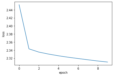
Epoch 1/10
860/860 [==============================] - 5s 5ms/step - loss: 2.4527
Epoch 2/10
860/860 [==============================] - 4s 5ms/step - loss: 2.3431
Epoch 3/10
860/860 [==============================] - 4s 4ms/step - loss: 2.3351
Epoch 4/10
860/860 [==============================] - 4s 4ms/step - loss: 2.3301
Epoch 5/10
860/860 [==============================] - 4s 5ms/step - loss: 2.3259
Epoch 6/10
860/860 [==============================] - 4s 4ms/step - loss: 2.3223
Epoch 7/10
860/860 [==============================] - 4s 5ms/step - loss: 2.3191
Epoch 8/10
860/860 [==============================] - 4s 4ms/step - loss: 2.3160
Epoch 9/10
860/860 [==============================] - 4s 4ms/step - loss: 2.3130
Epoch 10/10
860/860 [==============================] - 4s 5ms/step - loss: 2.3104

最後に学習履歴をプロットします。

plt.plot(history.history["loss"])
plt.ylabel("loss")
plt.xlabel("epoch")
plt.show()

 

学習された埋め込みの分析

movie_embeddings = model.get_layer("item_embeddings").get_weights()[0]
print("Embeddings shape:", movie_embeddings.shape)

Embeddings shape: (1406, 50)

 

関連する映画を見つける

query_movies と呼ばれる幾つかの映画を含むリストを定義します。

query_movies = [
    "Matrix, The (1999)",
    "Star Wars: Episode IV - A New Hope (1977)",
    "Lion King, The (1994)",
    "Terminator 2: Judgment Day (1991)",
    "Godfather, The (1972)",
]

query_movies で映画の埋め込みを取得します。

query_embeddings = []

for movie_title in query_movies:
    movieId = get_movie_id_by_title(movie_title)
    token_id = vocabulary_lookup[movieId]
    movie_embedding = movie_embeddings[token_id]
    query_embeddings.append(movie_embedding)

query_embeddings = np.array(query_embeddings)

query_movies と総ての他の映画の間の埋め込み間の コサイン類似度 を計算してから、各々のために top k を選択します。

similarities = tf.linalg.matmul(
    tf.math.l2_normalize(query_embeddings),
    tf.math.l2_normalize(movie_embeddings),
    transpose_b=True,
)

_, indices = tf.math.top_k(similarities, k=5)
indices = indices.numpy().tolist()

query_movies の top 関連映画を表示します。

for idx, title in enumerate(query_movies):
    print(title)
    print("".rjust(len(title), "-"))
    similar_tokens = indices[idx]
    for token in similar_tokens:
        similar_movieId = vocabulary[token]
        similar_title = get_movie_title_by_id(similar_movieId)
        print(f"- {similar_title}")
    print()

Matrix, The (1999)
------------------
- Matrix, The (1999)
- Raiders of the Lost Ark (Indiana Jones and the Raiders of the Lost Ark) (1981)
- Schindler's List (1993)
- Star Wars: Episode IV - A New Hope (1977)
- Lord of the Rings: The Fellowship of the Ring, The (2001)

Star Wars: Episode IV - A New Hope (1977)
-----------------------------------------
- Star Wars: Episode IV - A New Hope (1977)
- Schindler's List (1993)
- Raiders of the Lost Ark (Indiana Jones and the Raiders of the Lost Ark) (1981)
- Matrix, The (1999)
- Pulp Fiction (1994)

Lion King, The (1994)
---------------------
- Lion King, The (1994)
- Jurassic Park (1993)
- Independence Day (a.k.a. ID4) (1996)
- Beauty and the Beast (1991)
- Mrs. Doubtfire (1993)

Terminator 2: Judgment Day (1991)
---------------------------------
- Schindler's List (1993)
- Jurassic Park (1993)
- Terminator 2: Judgment Day (1991)
- Star Wars: Episode IV - A New Hope (1977)
- Back to the Future (1985)

Godfather, The (1972)
---------------------
- Apocalypse Now (1979)
- Fargo (1996)
- Godfather, The (1972)
- Schindler's List (1993)
- Casablanca (1942)

 

Embedding Projector を使用して埋め込みを可視化する

import io

out_v = io.open("embeddings.tsv", "w", encoding="utf-8")
out_m = io.open("metadata.tsv", "w", encoding="utf-8")

for idx, movie_id in enumerate(vocabulary[1:]):
    movie_title = list(movies[movies.movieId == movie_id].title)[0]
    vector = movie_embeddings[idx]
    out_v.write("\t".join([str(x) for x in vector]) + "\n")
    out_m.write(movie_title + "\n")

out_v.close()
out_m.close()

Embedding Projector で取得した埋め込みを分析するために embeddings.tsv と metadata.tsv をダウンロードします。

HuggingFace で利用可能なサンプル :

• Trained Model
  

• Demo

以上