Keras 2 : examples : 画像の類似性検索のためのメトリック学習 (翻訳/解説)
翻訳 : (株)クラスキャット セールスインフォメーション
作成日時 : 11/27/2021 (keras 2.7.0)
* 本ページは、Keras の以下のドキュメントを翻訳した上で適宜、補足説明したものです:
- Code examples : Computer Vision : Metric learning for image similarity search (Author: Mat Kelcey)
* サンプルコードの動作確認はしておりますが、必要な場合には適宜、追加改変しています。
* ご自由にリンクを張って頂いてかまいませんが、sales-info@classcat.com までご一報いただけると嬉しいです。

- 人工知能研究開発支援
- 人工知能研修サービス(経営者層向けオンサイト研修)
- テクニカルコンサルティングサービス
- 実証実験(プロトタイプ構築)
- アプリケーションへの実装
- 人工知能研修サービス
- PoC(概念実証)を失敗させないための支援
- テレワーク & オンライン授業を支援
- お住まいの地域に関係なく Web ブラウザからご参加頂けます。事前登録 が必要ですのでご注意ください。
- ウェビナー運用には弊社製品「ClassCat® Webinar」を利用しています。
◆ お問合せ : 本件に関するお問い合わせ先は下記までお願いいたします。
- 株式会社クラスキャット セールス・マーケティング本部 セールス・インフォメーション
- E-Mail:sales-info@classcat.com ; WebSite: www.classcat.com ; Facebook

Keras 2 : examples : 画像の類似性検索のためのメトリック学習
Description: CIFAR-10 画像上の類似性メトリック学習を使用するサンプル。
概要
メトリック学習は、(訓練スキームにより定義された) 「類似の」入力が互いに近く配置されるように、入力を高次元空間に埋め込めるモデルを訓練することを目的としています。一度訓練されたこれらのモデルはそのような類似性が有用であるような下流システムのための埋め込みを生成できます ; 例としては検索のためのランキングシグナルや、別の教師あり問題のための事前訓練済みの埋め込みモデルの形式を含みます。
メトリック学習の詳細な概要については以下を参照してください :
セットアップ
import random
import matplotlib.pyplot as plt
import numpy as np
import tensorflow as tf
from collections import defaultdict
from PIL import Image
from sklearn.metrics import ConfusionMatrixDisplay
from tensorflow import keras
from tensorflow.keras import layers
データセット
このサンプルのためには CIFAR-10 データセットを使用していきます。
from tensorflow.keras.datasets import cifar10

(x_train, y_train), (x_test, y_test) = cifar10.load_data()

x_train = x_train.astype("float32") / 255.0
y_train = np.squeeze(y_train)
x_test = x_test.astype("float32") / 255.0
y_test = np.squeeze(y_test)
データセットの感覚を得るために 25 のランダムサンプルのグリッドを可視化できます。
height_width = 32


def show_collage(examples):
    box_size = height_width + 2
    num_rows, num_cols = examples.shape[:2]

    collage = Image.new(
        mode="RGB",
        size=(num_cols * box_size, num_rows * box_size),
        color=(250, 250, 250),
    )
    for row_idx in range(num_rows):
        for col_idx in range(num_cols):
            array = (np.array(examples[row_idx, col_idx]) * 255).astype(np.uint8)
            collage.paste(
                Image.fromarray(array), (col_idx * box_size, row_idx * box_size)
            )

    # Double size for visualisation.
    collage = collage.resize((2 * num_cols * box_size, 2 * num_rows * box_size))
    return collage


# Show a collage of 5x5 random images.
sample_idxs = np.random.randint(0, 50000, size=(5, 5))
examples = x_train[sample_idxs]
show_collage(examples)

メトリック学習は訓練データを明示的な (X, y) ペアとして提供するのではなく代わりに、類似性を表現したい方法で関係する複数のインスタンスを使用します。このサンプルでは類似性を表現するために同じクラスのインスタンスを使用します ; 単一の訓練インスタンスは 1 つの画像ではなく、同じクラスの画像のペアになります。このペアの画像を参照するとき、アンカー (ランダムに選択された画像) とポジティブ (同じクラスのランダムに選択された別の画像) の一般的なメトリック学習名を使用します。
これを容易にするため、クラスからクラスのインスタンスにマップする検索の形式を構築する必要があります。訓練のためのデータを生成するときこの検索からサンプリングします。
class_idx_to_train_idxs = defaultdict(list)
for y_train_idx, y in enumerate(y_train):
    class_idx_to_train_idxs[y].append(y_train_idx)

class_idx_to_test_idxs = defaultdict(list)
for y_test_idx, y in enumerate(y_test):
    class_idx_to_test_idxs[y].append(y_test_idx)
この例のために、訓練への最も単純なアプローチを使用しています ; バッチはクラスに渡る (anchor, positive) ペアから成ります。学習の目標はアンカーとポジティブのペアを一緒に近づけ、そしてバッチの他のインスタンスから遠ざけることです。この場合、バッチサイズはクラス数により決定されます ; CIFAR-10 についてはこれは 10 です。
num_classes = 10


class AnchorPositivePairs(keras.utils.Sequence):
    def __init__(self, num_batchs):
        self.num_batchs = num_batchs

    def __len__(self):
        return self.num_batchs

    def __getitem__(self, _idx):
        x = np.empty((2, num_classes, height_width, height_width, 3), dtype=np.float32)
        for class_idx in range(num_classes):
            examples_for_class = class_idx_to_train_idxs[class_idx]
            anchor_idx = random.choice(examples_for_class)
            positive_idx = random.choice(examples_for_class)
            while positive_idx == anchor_idx:
                positive_idx = random.choice(examples_for_class)
            x[0, class_idx] = x_train[anchor_idx]
            x[1, class_idx] = x_train[positive_idx]
        return x
バッチをもう一つのコラージュで可視化できます。上の行は 10 クラスからランダムに選択されたアンカーで、下の行は対応する 10 のポジティブを表示しています。
examples = next(iter(AnchorPositivePairs(num_batchs=1)))

show_collage(examples)

埋め込みモデル
train_step を持つカスタムモデルを定義します、これは最初にアンカーとポジティブの両方を埋め込みそして softmax に対するロジットとしてペア毎のドット積を使用します。
class EmbeddingModel(keras.Model):
    def train_step(self, data):
        # Note: Workaround for open issue, to be removed.
        if isinstance(data, tuple):
            data = data[0]
        anchors, positives = data[0], data[1]

        with tf.GradientTape() as tape:
            # Run both anchors and positives through model.
            anchor_embeddings = self(anchors, training=True)
            positive_embeddings = self(positives, training=True)

            # Calculate cosine similarity between anchors and positives. As they have
            # been normalised this is just the pair wise dot products.
            similarities = tf.einsum(
                "ae,pe->ap", anchor_embeddings, positive_embeddings
            )

            # Since we intend to use these as logits we scale them by a temperature.
            # This value would normally be chosen as a hyper parameter.
            temperature = 0.2
            similarities /= temperature

            # We use these similarities as logits for a softmax. The labels for
            # this call are just the sequence [0, 1, 2, ..., num_classes] since we
            # want the main diagonal values, which correspond to the anchor/positive
            # pairs, to be high. This loss will move embeddings for the
            # anchor/positive pairs together and move all other pairs apart.
            sparse_labels = tf.range(num_classes)
            loss = self.compiled_loss(sparse_labels, similarities)

        # Calculate gradients and apply via optimizer.
        gradients = tape.gradient(loss, self.trainable_variables)
        self.optimizer.apply_gradients(zip(gradients, self.trainable_variables))

        # Update and return metrics (specifically the one for the loss value).
        self.compiled_metrics.update_state(sparse_labels, similarities)
        return {m.name: m.result() for m in self.metrics}
次に画像から埋め込みへマップするアーキテクチャを説明します。このモデルは単純に 2d 畳み込みにグルーバルプーリングが続くシークエンスから構成され、最後に埋め込み空間への線形射影を持ちます。メトリック学習で一般的なように、類似性を測定するために単純なドット積を使用できるように埋め込みを正規化します。単純性のためにこのモデルは意図的に小さくしてあります。
inputs = layers.Input(shape=(height_width, height_width, 3))
x = layers.Conv2D(filters=32, kernel_size=3, strides=2, activation="relu")(inputs)
x = layers.Conv2D(filters=64, kernel_size=3, strides=2, activation="relu")(x)
x = layers.Conv2D(filters=128, kernel_size=3, strides=2, activation="relu")(x)
x = layers.GlobalAveragePooling2D()(x)
embeddings = layers.Dense(units=8, activation=None)(x)
embeddings = tf.nn.l2_normalize(embeddings, axis=-1)

model = EmbeddingModel(inputs, embeddings)
最後に訓練を実行します。Google Colab GPU インスタンスでこれはおよそ 1 分間かかります。
model.compile(
    optimizer=keras.optimizers.Adam(learning_rate=1e-3),
    loss=keras.losses.SparseCategoricalCrossentropy(from_logits=True),
)

history = model.fit(AnchorPositivePairs(num_batchs=1000), epochs=20)

plt.plot(history.history["loss"])
plt.show()
Epoch 1/20
1000/1000 [==============================] - 4s 4ms/step - loss: 2.2475
Epoch 2/20
1000/1000 [==============================] - 5s 5ms/step - loss: 2.1246
Epoch 3/20
1000/1000 [==============================] - 7s 7ms/step - loss: 2.0519
Epoch 4/20
1000/1000 [==============================] - 8s 8ms/step - loss: 2.0011
Epoch 5/20
1000/1000 [==============================] - 9s 9ms/step - loss: 1.9601
Epoch 6/20
1000/1000 [==============================] - 9s 9ms/step - loss: 1.9214
Epoch 7/20
1000/1000 [==============================] - 9s 9ms/step - loss: 1.9094
Epoch 8/20
1000/1000 [==============================] - 10s 10ms/step - loss: 1.8669
Epoch 9/20
1000/1000 [==============================] - 10s 10ms/step - loss: 1.8462
Epoch 10/20
1000/1000 [==============================] - 10s 10ms/step - loss: 1.8095
Epoch 11/20
1000/1000 [==============================] - 10s 10ms/step - loss: 1.7854
Epoch 12/20
1000/1000 [==============================] - 11s 11ms/step - loss: 1.7595
Epoch 13/20
1000/1000 [==============================] - 11s 11ms/step - loss: 1.7538
Epoch 14/20
1000/1000 [==============================] - 11s 11ms/step - loss: 1.7198
Epoch 15/20
 906/1000 [==========================>...] - ETA: 1s - loss: 1.7017
(訳者注: 実験結果)
Epoch 1/20
1000/1000 [==============================] - 15s 6ms/step - loss: 2.2602
Epoch 2/20
1000/1000 [==============================] - 6s 6ms/step - loss: 2.1384
Epoch 3/20
1000/1000 [==============================] - 6s 6ms/step - loss: 2.0423
Epoch 4/20
1000/1000 [==============================] - 6s 6ms/step - loss: 2.0288
Epoch 5/20
1000/1000 [==============================] - 6s 6ms/step - loss: 1.9969
Epoch 6/20
1000/1000 [==============================] - 6s 6ms/step - loss: 1.9725
Epoch 7/20
1000/1000 [==============================] - 6s 6ms/step - loss: 1.9510
Epoch 8/20
1000/1000 [==============================] - 6s 6ms/step - loss: 1.9403
Epoch 9/20
1000/1000 [==============================] - 6s 6ms/step - loss: 1.9169
Epoch 10/20
1000/1000 [==============================] - 6s 6ms/step - loss: 1.8850
Epoch 11/20
1000/1000 [==============================] - 6s 6ms/step - loss: 1.8773
Epoch 12/20
1000/1000 [==============================] - 6s 6ms/step - loss: 1.8579
Epoch 13/20
1000/1000 [==============================] - 6s 6ms/step - loss: 1.8489
Epoch 14/20
1000/1000 [==============================] - 6s 6ms/step - loss: 1.8312
Epoch 15/20
1000/1000 [==============================] - 6s 6ms/step - loss: 1.8074
Epoch 16/20
1000/1000 [==============================] - 6s 6ms/step - loss: 1.7890
Epoch 17/20
1000/1000 [==============================] - 6s 6ms/step - loss: 1.7878
Epoch 18/20
1000/1000 [==============================] - 6s 6ms/step - loss: 1.7627
Epoch 19/20
1000/1000 [==============================] - 6s 6ms/step - loss: 1.7431
Epoch 20/20
1000/1000 [==============================] - 6s 6ms/step - loss: 1.7280

テスト
(モデルを) テストセットに適用して埋め込み空間の近傍を考えることにより、このモデルの品質をレビューできます。
最初にテストセットを埋め込みそして総ての近傍を計算します。埋め込みは単位長さですからドット積を通してコサイン類似度を計算できることを思い出してください。
near_neighbours_per_example = 10

embeddings = model.predict(x_test)
gram_matrix = np.einsum("ae,be->ab", embeddings, embeddings)
near_neighbours = np.argsort(gram_matrix.T)[:, -(near_neighbours_per_example + 1) :]
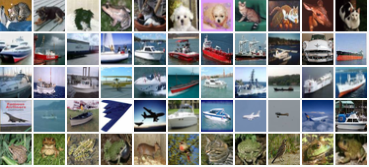
これらの埋め込みの視覚的な確認として、5 つのランダムサンプルに対する近傍のコラージュを構築できます。下の画像の最初のカラムがランダムに選択された画像で、続く 10 列が類似度の順で近傍を示しています。
num_collage_examples = 5

examples = np.empty(
    (
        num_collage_examples,
        near_neighbours_per_example + 1,
        height_width,
        height_width,
        3,
    ),
    dtype=np.float32,
)
for row_idx in range(num_collage_examples):
    examples[row_idx, 0] = x_test[row_idx]
    anchor_near_neighbours = reversed(near_neighbours[row_idx][:-1])
    for col_idx, nn_idx in enumerate(anchor_near_neighbours):
        examples[row_idx, col_idx + 1] = x_test[nn_idx]

show_collage(examples)
混同行列の視点で近傍の正しさを考えることにより、パフォーマンスの定量的なビューを得ることもできます。
10 クラスの各々から 10 サンプルをサンプリングしてそれらの近傍を予測の形で考えましょう ; つまり、サンプルとその近傍が同じクラスを共有しているか?ということです。
各動物クラスは一般に上手く遂行していて、他の動物クラスと最も混同しています。乗り物 (= vehicle) のクラスも同じパターンに従っています。
confusion_matrix = np.zeros((num_classes, num_classes))

# For each class.
for class_idx in range(num_classes):
    # Consider 10 examples.
    example_idxs = class_idx_to_test_idxs[class_idx][:10]
    for y_test_idx in example_idxs:
        # And count the classes of its near neighbours.
        for nn_idx in near_neighbours[y_test_idx][:-1]:
            nn_class_idx = y_test[nn_idx]
            confusion_matrix[class_idx, nn_class_idx] += 1

# Display a confusion matrix.
labels = [
    "Airplane",
    "Automobile",
    "Bird",
    "Cat",
    "Deer",
    "Dog",
    "Frog",
    "Horse",
    "Ship",
    "Truck",
]
disp = ConfusionMatrixDisplay(confusion_matrix=confusion_matrix, display_labels=labels)
disp.plot(include_values=True, cmap="viridis", ax=None, xticks_rotation="vertical")
plt.show()


以上