Keras 2 : examples : Siamese ネットワークを対照損失で使用した画像類似性推定 (翻訳/解説)

翻訳 : (株)クラスキャット セールスインフォメーション
作成日時 : 12/14/2021 (keras 2.7.0)

* 本ページは、Keras の以下のドキュメントを翻訳した上で適宜、補足説明したものです：

• Code examples : Computer Vision : Image similarity estimation using a Siamese Network with a contrastive loss (Author: Mehdi)

* サンプルコードの動作確認はしておりますが、必要な場合には適宜、追加改変しています。
* ご自由にリンクを張って頂いてかまいませんが、sales-info@classcat.com までご一報いただけると嬉しいです。

 

 

 

Keras 2 : examples : Siamese ネットワークを対照損失で使用した画像類似性推定

Description: 対照損失で訓練された siamese ネットワークを使用した類似性学習。

 

イントロダクション

Siamese ネットワーク は 2 つまたはそれ以上の姉妹 (= sister) ネットワーク間で重みを共有するニューラルネットワークで、それぞれがそれぞれの入力の埋め込みベクトルを生成します。

教師あり類似性学習では、次にネットワークは異なるクラスの入力の埋め込み間のコントラスト (距離) を最大化する一方で、類似クラスの埋め込み間の距離を最小化するために訓練され、訓練入力のクラス分割を反映した埋め込み空間という結果になります。

 

セットアップ

import random
import numpy as np
import tensorflow as tf
from tensorflow import keras
from tensorflow.keras import layers
import matplotlib.pyplot as plt

 

ハイパーパラメータ

epochs = 10
batch_size = 16
margin = 1  # Margin for constrastive loss.

 

MNIST データセットのロード

(x_train_val, y_train_val), (x_test, y_test) = keras.datasets.mnist.load_data()

# Change the data type to a floating point format
x_train_val = x_train_val.astype("float32")
x_test = x_test.astype("float32")

 

訓練と検証セットの定義

# Keep 50% of train_val  in validation set
x_train, x_val = x_train_val[:30000], x_train_val[30000:]
y_train, y_val = y_train_val[:30000], y_train_val[30000:]
del x_train_val, y_train_val

 

画像のペアの作成

異なるクラスの数字を識別するようにモデルを訓練します。例えば、数字 0 は残りの数字 (1 〜 9) と識別される必要があり、数字 1 は、0 と 2 〜 9 と識別される必要があります、等々。これを実行するため、クラス A (例えば、数字 0 に対して) から N 個のランダムな画像を選択して、それらを別のクラス B (例えば、数字 1 に対して) からの N 個のランダムな画像とペアリングします。そして、このプロセスを数字の総てのクラス (数字 9 まで) に対して反復できます。数字の 0 を他の数字とペアリングしたら、このプロセスを残りの数字 (1 〜 9) のための残りのクラスに対して反復できます。

def make_pairs(x, y):
    """Creates a tuple containing image pairs with corresponding label.

    Arguments:
        x: List containing images, each index in this list corresponds to one image.
        y: List containing labels, each label with datatype of `int`.

    Returns:
        Tuple containing two numpy arrays as (pairs_of_samples, labels),
        where pairs_of_samples' shape is (2len(x), 2,n_features_dims) and
        labels are a binary array of shape (2len(x)).
    """

    num_classes = max(y) + 1
    digit_indices = [np.where(y == i)[0] for i in range(num_classes)]

    pairs = []
    labels = []

    for idx1 in range(len(x)):
        # add a matching example
        x1 = x[idx1]
        label1 = y[idx1]
        idx2 = random.choice(digit_indices[label1])
        x2 = x[idx2]

        pairs += [[x1, x2]]
        labels += [1]

        # add a non-matching example
        label2 = random.randint(0, num_classes - 1)
        while label2 == label1:
            label2 = random.randint(0, num_classes - 1)

        idx2 = random.choice(digit_indices[label2])
        x2 = x[idx2]

        pairs += [[x1, x2]]
        labels += [0]

    return np.array(pairs), np.array(labels).astype("float32")


# make train pairs
pairs_train, labels_train = make_pairs(x_train, y_train)

# make validation pairs
pairs_val, labels_val = make_pairs(x_val, y_val)

# make test pairs
pairs_test, labels_test = make_pairs(x_test, y_test)

次を得ます :

pairs_train.shape = (60000, 2, 28, 28)

• 60,000 ペアを持ちます。
• 各ペアは 2 つの画像を持ちます。
• 各画像は shape (28, 28) です。

訓練ペアを分割します :

x_train_1 = pairs_train[:, 0]  # x_train_1.shape is (60000, 28, 28)
x_train_2 = pairs_train[:, 1]

検証ペアを分割します :

x_val_1 = pairs_val[:, 0]  # x_val_1.shape = (60000, 28, 28)
x_val_2 = pairs_val[:, 1]

テストペアを分割します :

x_test_1 = pairs_test[:, 0]  # x_test_1.shape = (20000, 28, 28)
x_test_2 = pairs_test[:, 1]

 

ペアとそれらのラベルを可視化する

def visualize(pairs, labels, to_show=6, num_col=3, predictions=None, test=False):
    """Creates a plot of pairs and labels, and prediction if it's test dataset.

    Arguments:
        pairs: Numpy Array, of pairs to visualize, having shape
               (Number of pairs, 2, 28, 28).
        to_show: Int, number of examples to visualize (default is 6)
                `to_show` must be an integral multiple of `num_col`.
                 Otherwise it will be trimmed if it is greater than num_col,
                 and incremented if if it is less then num_col.
        num_col: Int, number of images in one row - (default is 3)
                 For test and train respectively, it should not exceed 3 and 7.
        predictions: Numpy Array of predictions with shape (to_show, 1) -
                     (default is None)
                     Must be passed when test=True.
        test: Boolean telling whether the dataset being visualized is
              train dataset or test dataset - (default False).

    Returns:
        None.
    """

    # Define num_row
    # If to_show % num_col != 0
    #    trim to_show,
    #       to trim to_show limit num_row to the point where
    #       to_show % num_col == 0
    #
    # If to_show//num_col == 0
    #    then it means num_col is greater then to_show
    #    increment to_show
    #       to increment to_show set num_row to 1
    num_row = to_show // num_col if to_show // num_col != 0 else 1

    # `to_show` must be an integral multiple of `num_col`
    #  we found num_row and we have num_col
    #  to increment or decrement to_show
    #  to make it integral multiple of `num_col`
    #  simply set it equal to num_row * num_col
    to_show = num_row * num_col

    # Plot the images
    fig, axes = plt.subplots(num_row, num_col, figsize=(5, 5))
    for i in range(to_show):

        # If the number of rows is 1, the axes array is one-dimensional
        if num_row == 1:
            ax = axes[i % num_col]
        else:
            ax = axes[i // num_col, i % num_col]

        ax.imshow(tf.concat([pairs[i][0], pairs[i][1]], axis=1), cmap="gray")
        ax.set_axis_off()
        if test:
            ax.set_title("True: {} | Pred: {:.5f}".format(labels[i], predictions[i][0]))
        else:
            ax.set_title("Label: {}".format(labels[i]))
    if test:
        plt.tight_layout(rect=(0, 0, 1.9, 1.9), w_pad=0.0)
    else:
        plt.tight_layout(rect=(0, 0, 1.5, 1.5))
    plt.show()

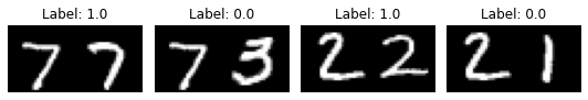
訓練ペアを調べる :

visualize(pairs_train[:-1], labels_train[:-1], to_show=4, num_col=4)

検証ペアを調べる :

visualize(pairs_val[:-1], labels_val[:-1], to_show=4, num_col=4)

テストペアを調べる :

visualize(pairs_test[:-1], labels_test[:-1], to_show=4, num_col=4)

 

モデルの定義

2 つの入力層があり、それぞれが独自のネットワークに繋がり、埋め込みを生成します。そして Lambda 層が ユークリッド距離 を使用してそれらをマージして、マージされた出力は最終的なネットワークに供給されます。

# Provided two tensors t1 and t2
# Euclidean distance = sqrt(sum(square(t1-t2)))
def euclidean_distance(vects):
    """Find the Euclidean distance between two vectors.

    Arguments:
        vects: List containing two tensors of same length.

    Returns:
        Tensor containing euclidean distance
        (as floating point value) between vectors.
    """

    x, y = vects
    sum_square = tf.math.reduce_sum(tf.math.square(x - y), axis=1, keepdims=True)
    return tf.math.sqrt(tf.math.maximum(sum_square, tf.keras.backend.epsilon()))


input = layers.Input((28, 28, 1))
x = tf.keras.layers.BatchNormalization()(input)
x = layers.Conv2D(4, (5, 5), activation="tanh")(x)
x = layers.AveragePooling2D(pool_size=(2, 2))(x)
x = layers.Conv2D(16, (5, 5), activation="tanh")(x)
x = layers.AveragePooling2D(pool_size=(2, 2))(x)
x = layers.Flatten()(x)

x = tf.keras.layers.BatchNormalization()(x)
x = layers.Dense(10, activation="tanh")(x)
embedding_network = keras.Model(input, x)


input_1 = layers.Input((28, 28, 1))
input_2 = layers.Input((28, 28, 1))

# As mentioned above, Siamese Network share weights between
# tower networks (sister networks). To allow this, we will use
# same embedding network for both tower networks.
tower_1 = embedding_network(input_1)
tower_2 = embedding_network(input_2)

merge_layer = layers.Lambda(euclidean_distance)([tower_1, tower_2])
normal_layer = tf.keras.layers.BatchNormalization()(merge_layer)
output_layer = layers.Dense(1, activation="sigmoid")(normal_layer)
siamese = keras.Model(inputs=[input_1, input_2], outputs=output_layer)

 

対照損失の定義

def loss(margin=1):
    """Provides 'constrastive_loss' an enclosing scope with variable 'margin'.

  Arguments:
      margin: Integer, defines the baseline for distance for which pairs
              should be classified as dissimilar. - (default is 1).

  Returns:
      'constrastive_loss' function with data ('margin') attached.
  """

    # Contrastive loss = mean( (1-true_value) * square(prediction) +
    #                         true_value * square( max(margin-prediction, 0) ))
    def contrastive_loss(y_true, y_pred):
        """Calculates the constrastive loss.

      Arguments:
          y_true: List of labels, each label is of type float32.
          y_pred: List of predictions of same length as of y_true,
                  each label is of type float32.

      Returns:
          A tensor containing constrastive loss as floating point value.
      """

        square_pred = tf.math.square(y_pred)
        margin_square = tf.math.square(tf.math.maximum(margin - (y_pred), 0))
        return tf.math.reduce_mean(
            (1 - y_true) * square_pred + (y_true) * margin_square
        )

    return contrastive_loss

 

対照損失でモデルのコンパイル

siamese.compile(loss=loss(margin=margin), optimizer="RMSprop", metrics=["accuracy"])
siamese.summary()

Model: "model_1"
__________________________________________________________________________________________________
Layer (type)                    Output Shape         Param #     Connected to                     
==================================================================================================
input_2 (InputLayer)            [(None, 28, 28, 1)]  0                                            
__________________________________________________________________________________________________
input_3 (InputLayer)            [(None, 28, 28, 1)]  0                                            
__________________________________________________________________________________________________
model (Functional)              (None, 10)           5318        input_2[0][0]                    
                                                                 input_3[0][0]                    
__________________________________________________________________________________________________
lambda (Lambda)                 (None, 1)            0           model[0][0]                      
                                                                 model[1][0]                      
__________________________________________________________________________________________________
batch_normalization_2 (BatchNor (None, 1)            4           lambda[0][0]                     
__________________________________________________________________________________________________
dense_1 (Dense)                 (None, 1)            2           batch_normalization_2[0][0]      
==================================================================================================
Total params: 5,324
Trainable params: 4,808
Non-trainable params: 516
__________________________________________________________________________________________________

 

モデルの訓練

history = siamese.fit(
    [x_train_1, x_train_2],
    labels_train,
    validation_data=([x_val_1, x_val_2], labels_val),
    batch_size=batch_size,
    epochs=epochs,
)

Epoch 1/10
3750/3750 [==============================] - 25s 6ms/step - loss: 0.1993 - accuracy: 0.6626 - val_loss: 0.0525 - val_accuracy: 0.9331
Epoch 2/10
3750/3750 [==============================] - 23s 6ms/step - loss: 0.0611 - accuracy: 0.9187 - val_loss: 0.0277 - val_accuracy: 0.9644
Epoch 3/10
3750/3750 [==============================] - 24s 6ms/step - loss: 0.0455 - accuracy: 0.9409 - val_loss: 0.0214 - val_accuracy: 0.9719
Epoch 4/10
3750/3750 [==============================] - 27s 7ms/step - loss: 0.0386 - accuracy: 0.9506 - val_loss: 0.0198 - val_accuracy: 0.9743
Epoch 5/10
3750/3750 [==============================] - 45s 12ms/step - loss: 0.0362 - accuracy: 0.9529 - val_loss: 0.0169 - val_accuracy: 0.9783
Epoch 6/10
2497/3750 [==================>...........] - ETA: 10s - loss: 0.0343 - accuracy: 0.9552

(訳者注 : 実験結果)

Epoch 1/10
3750/3750 [==============================] - 37s 7ms/step - loss: 0.0900 - accuracy: 0.8781 - val_loss: 0.0378 - val_accuracy: 0.9501
Epoch 2/10
3750/3750 [==============================] - 26s 7ms/step - loss: 0.0534 - accuracy: 0.9291 - val_loss: 0.0264 - val_accuracy: 0.9656
Epoch 3/10
3750/3750 [==============================] - 26s 7ms/step - loss: 0.0438 - accuracy: 0.9425 - val_loss: 0.0187 - val_accuracy: 0.9761
Epoch 4/10
3750/3750 [==============================] - 26s 7ms/step - loss: 0.0383 - accuracy: 0.9503 - val_loss: 0.0170 - val_accuracy: 0.9786
Epoch 5/10
3750/3750 [==============================] - 26s 7ms/step - loss: 0.0357 - accuracy: 0.9535 - val_loss: 0.0201 - val_accuracy: 0.9746
Epoch 6/10
3750/3750 [==============================] - 26s 7ms/step - loss: 0.0339 - accuracy: 0.9562 - val_loss: 0.0156 - val_accuracy: 0.9802
Epoch 7/10
3750/3750 [==============================] - 26s 7ms/step - loss: 0.0323 - accuracy: 0.9584 - val_loss: 0.0160 - val_accuracy: 0.9789
Epoch 8/10
3750/3750 [==============================] - 26s 7ms/step - loss: 0.0305 - accuracy: 0.9604 - val_loss: 0.0185 - val_accuracy: 0.9760
Epoch 9/10
3750/3750 [==============================] - 26s 7ms/step - loss: 0.0310 - accuracy: 0.9602 - val_loss: 0.0169 - val_accuracy: 0.9783
Epoch 10/10
3750/3750 [==============================] - 26s 7ms/step - loss: 0.0315 - accuracy: 0.9595 - val_loss: 0.0152 - val_accuracy: 0.9806

 

結果の可視化

def plt_metric(history, metric, title, has_valid=True):
    """Plots the given 'metric' from 'history'.

    Arguments:
        history: history attribute of History object returned from Model.fit.
        metric: Metric to plot, a string value present as key in 'history'.
        title: A string to be used as title of plot.
        has_valid: Boolean, true if valid data was passed to Model.fit else false.

    Returns:
        None.
    """
    plt.plot(history[metric])
    if has_valid:
        plt.plot(history["val_" + metric])
        plt.legend(["train", "validation"], loc="upper left")
    plt.title(title)
    plt.ylabel(metric)
    plt.xlabel("epoch")
    plt.show()


# Plot the accuracy
plt_metric(history=history.history, metric="accuracy", title="Model accuracy")

# Plot the constrastive loss
plt_metric(history=history.history, metric="loss", title="Constrastive Loss")

 

モデルの評価

results = siamese.evaluate([x_test_1, x_test_2], labels_test)
print("test loss, test acc:", results)

625/625 [==============================] - 3s 4ms/step - loss: 0.0150 - accuracy: 0.9810
test loss, test acc: [0.015001337975263596, 0.9810000061988831]

625/625 [==============================] - 2s 3ms/step - loss: 0.0125 - accuracy: 0.9834
test loss, test acc: [0.01245756447315216, 0.9834499955177307]

 

予測の可視化

predictions = siamese.predict([x_test_1, x_test_2])
visualize(pairs_test, labels_test, to_show=3, predictions=predictions, test=True)

以上