Keras 2 : examples : グラフデータ – 分子的性質のためのメッセージパッシング・ニューラルネット (MPNN) (翻訳/解説)

翻訳 : (株)クラスキャット セールスインフォメーション
作成日時 : 08/06/2022 (keras 2.9.0)

メッセージパッシングニューラルネットワーク(MPNN)による分子特性予測

* 本ページは、Keras の以下のドキュメントを翻訳した上で適宜、補足説明したものです：

• Code examples : Graph Data : Message-passing neural network (MPNN) for molecular property prediction (Author: akensert)

* サンプルコードの動作確認はしておりますが、必要な場合には適宜、追加改変しています。
* ご自由にリンクを張って頂いてかまいませんが、sales-info@classcat.com までご一報いただけると嬉しいです。

 

 

 

Keras 2 : examples : グラフデータ – 分子的性質のためのメッセージパッシング・ニューラルネット (MPNN)

Description : 血液脳関門 (= blood-brain barrier) 透過性 (= permeability) を予測する MPNN の実装。

 

イントロダクション

このチュートリアルでは、グラフ特性を予測するために _ メッセージパッシング・ニューラルネットワーク _ (MPNN) として知られるグラフニューラルネットワーク (GNN) のタイプを実装します。具体的には、血液脳関門透過性 (BBBP) として知られる分子的性質を予測するために MPNN を実装します。

動機 : 分子が無向グラフ G = (V, E) として自然に表現されるとき、ここで V は頂点 (ノード ; 原子) の集合で E はエッジ (結合) の集合、(MPNN のような) GNN が分子的性質を予測するために有用な方法であることが判明しています。

これまで、ランダムフォレスト、サポートベクターマシン 等のような、従来の方法が分子的特性を予測するために一般に使用されてきました。GNN とは対象的に、これらの従来のアプローチは分子量, 極性, 電荷, 炭素原子の数 etc. のような、事前計算された分子的特徴で動作することが多いです。これらの分子的特徴は様々な分子的性質に対して良い予測因子であることが分かっていますが、これらのより “raw”、”低位” な特徴上での演算は更に良いと示されると仮定されています。

 

References

近年、分子グラフを含む、グラフデータのためのニューラルネットワークを開発するために多くの努力が成されてきました。グラフニューラルネットワークの概要については、例えば、A Comprehensive Survey on Graph Neural Networks と Graph Neural Networks: A Review of Methods and Applications を見てください ; そしてこのチュートリアルで実装される特定のグラフニューラルネットワークについて更に読むには、Neural Message Passing for Quantum Chemistry と DeepChem’s MPNNModel を見てください。

 

セットアップ

RDKit と他の依存性のインストール

(下のテキストは このチュートリアル から引用)。

RDKit は C++ と Python で書かれたケモインフォマティクス (= cheminformatics) と機械学習ソフトウェアのコレクションです。このチュートリアルでは、RDKit は便利に効率的に SMILES を分子オブジェクトに変換し、それから原子と結合のセットを取得するために使用されます。

SMILES は与えられた分子の構造を ASCII 文字列の形式で表現します。SMILES 文字列はコンパクトなエンコーディングで、小さい分子に対しては、それは比較的可読です。分子の文字列としてのエンコーディングは、与えられたデータベース and/or web 検索の負担を軽減し、容易にします。RDKit は与えられた SMILES を分子オブジェクトに正確に変換するアルゴリズムを使用し、これは非常に多くの分子的性質/特徴を計算するために使用できます。

注意してください、RDKit は一般には Conda でインストールされます。しかし、rdkit_platform_wheels のおかげで、rdkit は今では (このチュートリアルのために) 次のように pip で容易にインストールできます :

pip -q install rdkit-pypi

そして csv ファイルの簡単で効率的な読み込みと可視化のために、以下のインストールが必要です :

pip -q install pandas
pip -q install Pillow
pip -q install matplotlib
pip -q install pydot
sudo apt-get -qq install graphviz

 

パッケージのインポート

import os

# Temporary suppress tf logs
os.environ["TF_CPP_MIN_LOG_LEVEL"] = "3"

import tensorflow as tf
from tensorflow import keras
from tensorflow.keras import layers
import numpy as np
import pandas as pd
import matplotlib.pyplot as plt
import warnings
from rdkit import Chem
from rdkit import RDLogger
from rdkit.Chem.Draw import IPythonConsole
from rdkit.Chem.Draw import MolsToGridImage

# Temporary suppress warnings and RDKit logs
warnings.filterwarnings("ignore")
RDLogger.DisableLog("rdApp.*")

np.random.seed(42)
tf.random.set_seed(42)

 

データセット

データセットについての情報は A Bayesian Approach to in Silico Blood-Brain Barrier Penetration Modeling と MoleculeNet: A Benchmark for Molecular Machine Learning で見つかります。データセットは MoleculeNet.org からダウンロードされます。

 

About

データセットは 2,050 分子を含みます。各分子は 名前、ラベル と SMILES 文字列を備えています。

血液脳関門 (BBB) は、血液を脳細胞外液から分離する膜で、殆どの薬物 (分子) が脳に到達することをブロックします。このため、BBBP は中枢神経系をターゲットとする新薬の開発を研究するのに重要であり続けています。このデータセットに対するラベルは二値 (1 or 0) で分子の透過性を示します。

csv_path = keras.utils.get_file(
    "BBBP.csv", "https://deepchemdata.s3-us-west-1.amazonaws.com/datasets/BBBP.csv"
)

df = pd.read_csv(csv_path, usecols=[1, 2, 3])
df.iloc[96:104]

 

特徴の定義

(後で必要となる) 原子と結合の特徴をエンコードするため、2 つのクラスを定義します : それぞれ AtomFeaturizer と BondFeaturizer です。

コードの行数をへらすため、つまりこのチュートリアルを短く簡潔にするため、一握りの (原子と結合) 特徴についてだけ考慮します : [原子の特徴] 記号 (元素), 価電子数, 水素結合の数, 軌道混成, [結合の特徴] (共有) 結合型, そして 共役。

class Featurizer:
    def __init__(self, allowable_sets):
        self.dim = 0
        self.features_mapping = {}
        for k, s in allowable_sets.items():
            s = sorted(list(s))
            self.features_mapping[k] = dict(zip(s, range(self.dim, len(s) + self.dim)))
            self.dim += len(s)

    def encode(self, inputs):
        output = np.zeros((self.dim,))
        for name_feature, feature_mapping in self.features_mapping.items():
            feature = getattr(self, name_feature)(inputs)
            if feature not in feature_mapping:
                continue
            output[feature_mapping[feature]] = 1.0
        return output


class AtomFeaturizer(Featurizer):
    def __init__(self, allowable_sets):
        super().__init__(allowable_sets)

    def symbol(self, atom):
        return atom.GetSymbol()

    def n_valence(self, atom):
        return atom.GetTotalValence()

    def n_hydrogens(self, atom):
        return atom.GetTotalNumHs()

    def hybridization(self, atom):
        return atom.GetHybridization().name.lower()


class BondFeaturizer(Featurizer):
    def __init__(self, allowable_sets):
        super().__init__(allowable_sets)
        self.dim += 1

    def encode(self, bond):
        output = np.zeros((self.dim,))
        if bond is None:
            output[-1] = 1.0
            return output
        output = super().encode(bond)
        return output

    def bond_type(self, bond):
        return bond.GetBondType().name.lower()

    def conjugated(self, bond):
        return bond.GetIsConjugated()


atom_featurizer = AtomFeaturizer(
    allowable_sets={
        "symbol": {"B", "Br", "C", "Ca", "Cl", "F", "H", "I", "N", "Na", "O", "P", "S"},
        "n_valence": {0, 1, 2, 3, 4, 5, 6},
        "n_hydrogens": {0, 1, 2, 3, 4},
        "hybridization": {"s", "sp", "sp2", "sp3"},
    }
)

bond_featurizer = BondFeaturizer(
    allowable_sets={
        "bond_type": {"single", "double", "triple", "aromatic"},
        "conjugated": {True, False},
    }
)

 

グラフの生成

SMILES から完全なグラフを生成可能とする前に、以下の関数を実装する必要があります :

1. molecule_from_smiles, これは入力として SMILES を取り分子オブジェクトを返します。これはすべて RDKit により処理されます。
   

2. graph_from_molecule, これは入力として分子オブジェクトを取り、3 タプル (atom_features, bond_features, pair_indices) として表現されるグラフを返します。このために先に定義されたクラスを利用します。

そして最後に、関数 graphs_from_smiles を実装できます、これは訓練, 検証とテストデータセットのすべての SMILES で関数 (1) そして続いて (2) を適用します。

Notice : このデータセットに対して scaffold 分割が勧められますが (こちら を参照)、簡略化のために、単純なランダム分割が実行されています。

def molecule_from_smiles(smiles):
    # MolFromSmiles(m, sanitize=True) should be equivalent to
    # MolFromSmiles(m, sanitize=False) -> SanitizeMol(m) -> AssignStereochemistry(m, ...)
    molecule = Chem.MolFromSmiles(smiles, sanitize=False)

    # If sanitization is unsuccessful, catch the error, and try again without
    # the sanitization step that caused the error
    flag = Chem.SanitizeMol(molecule, catchErrors=True)
    if flag != Chem.SanitizeFlags.SANITIZE_NONE:
        Chem.SanitizeMol(molecule, sanitizeOps=Chem.SanitizeFlags.SANITIZE_ALL ^ flag)

    Chem.AssignStereochemistry(molecule, cleanIt=True, force=True)
    return molecule


def graph_from_molecule(molecule):
    # Initialize graph
    atom_features = []
    bond_features = []
    pair_indices = []

    for atom in molecule.GetAtoms():
        atom_features.append(atom_featurizer.encode(atom))

        # Add self-loops
        pair_indices.append([atom.GetIdx(), atom.GetIdx()])
        bond_features.append(bond_featurizer.encode(None))

        for neighbor in atom.GetNeighbors():
            bond = molecule.GetBondBetweenAtoms(atom.GetIdx(), neighbor.GetIdx())
            pair_indices.append([atom.GetIdx(), neighbor.GetIdx()])
            bond_features.append(bond_featurizer.encode(bond))

    return np.array(atom_features), np.array(bond_features), np.array(pair_indices)


def graphs_from_smiles(smiles_list):
    # Initialize graphs
    atom_features_list = []
    bond_features_list = []
    pair_indices_list = []

    for smiles in smiles_list:
        molecule = molecule_from_smiles(smiles)
        atom_features, bond_features, pair_indices = graph_from_molecule(molecule)

        atom_features_list.append(atom_features)
        bond_features_list.append(bond_features)
        pair_indices_list.append(pair_indices)

    # Convert lists to ragged tensors for tf.data.Dataset later on
    return (
        tf.ragged.constant(atom_features_list, dtype=tf.float32),
        tf.ragged.constant(bond_features_list, dtype=tf.float32),
        tf.ragged.constant(pair_indices_list, dtype=tf.int64),
    )


# Shuffle array of indices ranging from 0 to 2049
permuted_indices = np.random.permutation(np.arange(df.shape[0]))

# Train set: 80 % of data
train_index = permuted_indices[: int(df.shape[0] * 0.8)]
x_train = graphs_from_smiles(df.iloc[train_index].smiles)
y_train = df.iloc[train_index].p_np

# Valid set: 19 % of data
valid_index = permuted_indices[int(df.shape[0] * 0.8) : int(df.shape[0] * 0.99)]
x_valid = graphs_from_smiles(df.iloc[valid_index].smiles)
y_valid = df.iloc[valid_index].p_np

# Test set: 1 % of data
test_index = permuted_indices[int(df.shape[0] * 0.99) :]
x_test = graphs_from_smiles(df.iloc[test_index].smiles)
y_test = df.iloc[test_index].p_np

 

関数のテスト

print(f"Name:\t{df.name[100]}\nSMILES:\t{df.smiles[100]}\nBBBP:\t{df.p_np[100]}")
molecule = molecule_from_smiles(df.iloc[100].smiles)
print("Molecule:")
molecule

Name:   acetylsalicylate
SMILES: CC(=O)Oc1ccccc1C(O)=O
BBBP:   0
Molecule:

graph = graph_from_molecule(molecule)
print("Graph (including self-loops):")
print("\tatom features\t", graph[0].shape)
print("\tbond features\t", graph[1].shape)
print("\tpair indices\t", graph[2].shape)

Graph (including self-loops):
    atom features    (13, 29)
    bond features    (39, 7)
    pair indices     (39, 2)

 

tf.data.Dataset の作成

このチュートリアルでは、MPNN 実装は (イテレーション毎に) 入力として単一グラフを取ります。従って、(sub) グラフ (分子) が与えられたとき、それらを単一グラフにマージする必要があります (このグラフをグローバルグラフとして参照します)。このグローバルグラフは非連結 (= disconnected) グラフで、各サブグラフは他のサブグラフから完全に分離しています。

def prepare_batch(x_batch, y_batch):
    """Merges (sub)graphs of batch into a single global (disconnected) graph
    """

    atom_features, bond_features, pair_indices = x_batch

    # Obtain number of atoms and bonds for each graph (molecule)
    num_atoms = atom_features.row_lengths()
    num_bonds = bond_features.row_lengths()

    # Obtain partition indices (molecule_indicator), which will be used to
    # gather (sub)graphs from global graph in model later on
    molecule_indices = tf.range(len(num_atoms))
    molecule_indicator = tf.repeat(molecule_indices, num_atoms)

    # Merge (sub)graphs into a global (disconnected) graph. Adding 'increment' to
    # 'pair_indices' (and merging ragged tensors) actualizes the global graph
    gather_indices = tf.repeat(molecule_indices[:-1], num_bonds[1:])
    increment = tf.cumsum(num_atoms[:-1])
    increment = tf.pad(tf.gather(increment, gather_indices), [(num_bonds[0], 0)])
    pair_indices = pair_indices.merge_dims(outer_axis=0, inner_axis=1).to_tensor()
    pair_indices = pair_indices + increment[:, tf.newaxis]
    atom_features = atom_features.merge_dims(outer_axis=0, inner_axis=1).to_tensor()
    bond_features = bond_features.merge_dims(outer_axis=0, inner_axis=1).to_tensor()

    return (atom_features, bond_features, pair_indices, molecule_indicator), y_batch


def MPNNDataset(X, y, batch_size=32, shuffle=False):
    dataset = tf.data.Dataset.from_tensor_slices((X, (y)))
    if shuffle:
        dataset = dataset.shuffle(1024)
    return dataset.batch(batch_size).map(prepare_batch, -1).prefetch(-1)

 

モデル

MPNN モデルは様々な shape と形式をとることができます。このチュートリアルでは、オリジナル論文 Neural Message Passing for Quantum Chemistry と DeepChem の MPNNModel に基づいて MPNN を実装します。このチュートリアルの MPNN は 3 つのステージから構成されます : メッセージパッシング, readout (読み出し) と分類です。

 

メッセージ・パッシング

メッセージパッシング・ステップ自身は 2 つのパートから成ります :

1. エッジネットワーク、これは v の 1-hop 近傍 w_{i} から v へその間のエッジ特徴量 (e_{vw_{i}}) に基づいてメッセージを渡し、更新されたノード (状態) v’ という結果になります。w_{i} は v の i:th 近傍を示します。
   

2. gated リカレント・ユニット (GRU), これは入力として最新のノード状態を取り、前のノード状態に基づいてそれを更新します。換言すれば、最新のノード状態は GRU への入力としてサーブし、一方で前のノード状態は GRU のメモリ状態内に組み込まれます。これは情報が一つのノード状態 (e.g., v) から別の (e.g., v”) に移動することを可能にします。

重要なことは、ステップ (1) と (2) は k ステップ繰り返され、そして各ステップ 1…k で、v からの集約情報の範囲 (= radius) (or hop の数) は 1 ずつ増えることです。

class EdgeNetwork(layers.Layer):
    def build(self, input_shape):
        self.atom_dim = input_shape[0][-1]
        self.bond_dim = input_shape[1][-1]
        self.kernel = self.add_weight(
            shape=(self.bond_dim, self.atom_dim * self.atom_dim),
            initializer="glorot_uniform",
            name="kernel",
        )
        self.bias = self.add_weight(
            shape=(self.atom_dim * self.atom_dim), initializer="zeros", name="bias",
        )
        self.built = True

    def call(self, inputs):
        atom_features, bond_features, pair_indices = inputs

        # Apply linear transformation to bond features
        bond_features = tf.matmul(bond_features, self.kernel) + self.bias

        # Reshape for neighborhood aggregation later
        bond_features = tf.reshape(bond_features, (-1, self.atom_dim, self.atom_dim))

        # Obtain atom features of neighbors
        atom_features_neighbors = tf.gather(atom_features, pair_indices[:, 1])
        atom_features_neighbors = tf.expand_dims(atom_features_neighbors, axis=-1)

        # Apply neighborhood aggregation
        transformed_features = tf.matmul(bond_features, atom_features_neighbors)
        transformed_features = tf.squeeze(transformed_features, axis=-1)
        aggregated_features = tf.math.unsorted_segment_sum(
            transformed_features,
            pair_indices[:, 0],
            num_segments=tf.shape(atom_features)[0],
        )
        return aggregated_features


class MessagePassing(layers.Layer):
    def __init__(self, units, steps=4, **kwargs):
        super().__init__(**kwargs)
        self.units = units
        self.steps = steps

    def build(self, input_shape):
        self.atom_dim = input_shape[0][-1]
        self.message_step = EdgeNetwork()
        self.pad_length = max(0, self.units - self.atom_dim)
        self.update_step = layers.GRUCell(self.atom_dim + self.pad_length)
        self.built = True

    def call(self, inputs):
        atom_features, bond_features, pair_indices = inputs

        # Pad atom features if number of desired units exceeds atom_features dim.
        # Alternatively, a dense layer could be used here.
        atom_features_updated = tf.pad(atom_features, [(0, 0), (0, self.pad_length)])

        # Perform a number of steps of message passing
        for i in range(self.steps):
            # Aggregate information from neighbors
            atom_features_aggregated = self.message_step(
                [atom_features_updated, bond_features, pair_indices]
            )

            # Update node state via a step of GRU
            atom_features_updated, _ = self.update_step(
                atom_features_aggregated, atom_features_updated
            )
        return atom_features_updated

 

Readout (読み出し)

メッセージパッシング手続きが終了するとき、k-step 集約されたノード状態は (バッチの各分離に対応して) サブグラフに分割されて、続いてグラフレベルの埋め込みに reduce されます。オリジナルの論文 では、set-to-set 層 がこの目的で使用されました。しかしこのチュートリアルでは、transformer エンコーダ + 平均プーリングが使用さます。具体的には :

• k-ステップ集約ノード状態は (バッチの各分子に対応して) サブグラフに分割されます ;
  

• そして各サブグラフは最大ノード数を持つサブグラフにマッチするようにパディングされ、tf.stack(…) が続きます ;
  

• サブグラフ (各サブグラフはノード状態のセットを含む) をエンコードする (stacked padded) テンソルはパディングが訓練を妨げないことを確実にするためにマスクされます ;
  

• 最後に、テンソルが transformer に渡され平均プーリングが続きます。

class PartitionPadding(layers.Layer):
    def __init__(self, batch_size, **kwargs):
        super().__init__(**kwargs)
        self.batch_size = batch_size

    def call(self, inputs):

        atom_features, molecule_indicator = inputs

        # Obtain subgraphs
        atom_features_partitioned = tf.dynamic_partition(
            atom_features, molecule_indicator, self.batch_size
        )

        # Pad and stack subgraphs
        num_atoms = [tf.shape(f)[0] for f in atom_features_partitioned]
        max_num_atoms = tf.reduce_max(num_atoms)
        atom_features_stacked = tf.stack(
            [
                tf.pad(f, [(0, max_num_atoms - n), (0, 0)])
                for f, n in zip(atom_features_partitioned, num_atoms)
            ],
            axis=0,
        )

        # Remove empty subgraphs (usually for last batch in dataset)
        gather_indices = tf.where(tf.reduce_sum(atom_features_stacked, (1, 2)) != 0)
        gather_indices = tf.squeeze(gather_indices, axis=-1)
        return tf.gather(atom_features_stacked, gather_indices, axis=0)


class TransformerEncoderReadout(layers.Layer):
    def __init__(
        self, num_heads=8, embed_dim=64, dense_dim=512, batch_size=32, **kwargs
    ):
        super().__init__(**kwargs)

        self.partition_padding = PartitionPadding(batch_size)
        self.attention = layers.MultiHeadAttention(num_heads, embed_dim)
        self.dense_proj = keras.Sequential(
            [layers.Dense(dense_dim, activation="relu"), layers.Dense(embed_dim),]
        )
        self.layernorm_1 = layers.LayerNormalization()
        self.layernorm_2 = layers.LayerNormalization()
        self.average_pooling = layers.GlobalAveragePooling1D()

    def call(self, inputs):
        x = self.partition_padding(inputs)
        padding_mask = tf.reduce_any(tf.not_equal(x, 0.0), axis=-1)
        padding_mask = padding_mask[:, tf.newaxis, tf.newaxis, :]
        attention_output = self.attention(x, x, attention_mask=padding_mask)
        proj_input = self.layernorm_1(x + attention_output)
        proj_output = self.layernorm_2(proj_input + self.dense_proj(proj_input))
        return self.average_pooling(proj_output)

 

メッセージパッシング・ニューラルネットワーク (MPNN)

MPNN モデルを完成させるときです。メッセージパッシングと readout に加えて、BBBP の予測を行なうために 2 層分類ネットワークが実装されます。

def MPNNModel(
    atom_dim,
    bond_dim,
    batch_size=32,
    message_units=64,
    message_steps=4,
    num_attention_heads=8,
    dense_units=512,
):

    atom_features = layers.Input((atom_dim), dtype="float32", name="atom_features")
    bond_features = layers.Input((bond_dim), dtype="float32", name="bond_features")
    pair_indices = layers.Input((2), dtype="int32", name="pair_indices")
    molecule_indicator = layers.Input((), dtype="int32", name="molecule_indicator")

    x = MessagePassing(message_units, message_steps)(
        [atom_features, bond_features, pair_indices]
    )

    x = TransformerEncoderReadout(
        num_attention_heads, message_units, dense_units, batch_size
    )([x, molecule_indicator])

    x = layers.Dense(dense_units, activation="relu")(x)
    x = layers.Dense(1, activation="sigmoid")(x)

    model = keras.Model(
        inputs=[atom_features, bond_features, pair_indices, molecule_indicator],
        outputs=[x],
    )
    return model


mpnn = MPNNModel(
    atom_dim=x_train[0][0][0].shape[0], bond_dim=x_train[1][0][0].shape[0],
)

mpnn.compile(
    loss=keras.losses.BinaryCrossentropy(),
    optimizer=keras.optimizers.Adam(learning_rate=5e-4),
    metrics=[keras.metrics.AUC(name="AUC")],
)

keras.utils.plot_model(mpnn, show_dtype=True, show_shapes=True)

 

訓練

train_dataset = MPNNDataset(x_train, y_train)
valid_dataset = MPNNDataset(x_valid, y_valid)
test_dataset = MPNNDataset(x_test, y_test)

history = mpnn.fit(
    train_dataset,
    validation_data=valid_dataset,
    epochs=40,
    verbose=2,
    class_weight={0: 2.0, 1: 0.5},
)

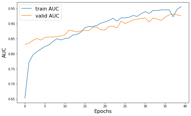
plt.figure(figsize=(10, 6))
plt.plot(history.history["AUC"], label="train AUC")
plt.plot(history.history["val_AUC"], label="valid AUC")
plt.xlabel("Epochs", fontsize=16)
plt.ylabel("AUC", fontsize=16)
plt.legend(fontsize=16)

Epoch 1/40
52/52 - 26s - loss: 0.5572 - AUC: 0.6527 - val_loss: 0.4660 - val_AUC: 0.8312 - 26s/epoch - 501ms/step
Epoch 2/40
52/52 - 22s - loss: 0.4817 - AUC: 0.7713 - val_loss: 0.6889 - val_AUC: 0.8351 - 22s/epoch - 416ms/step
Epoch 3/40
52/52 - 24s - loss: 0.4611 - AUC: 0.7960 - val_loss: 0.5863 - val_AUC: 0.8444 - 24s/epoch - 457ms/step
Epoch 4/40
52/52 - 19s - loss: 0.4493 - AUC: 0.8069 - val_loss: 0.5059 - val_AUC: 0.8509 - 19s/epoch - 372ms/step
Epoch 5/40
52/52 - 21s - loss: 0.4420 - AUC: 0.8155 - val_loss: 0.4965 - val_AUC: 0.8454 - 21s/epoch - 405ms/step
Epoch 6/40
52/52 - 22s - loss: 0.4344 - AUC: 0.8243 - val_loss: 0.5307 - val_AUC: 0.8540 - 22s/epoch - 419ms/step
Epoch 7/40
52/52 - 26s - loss: 0.4301 - AUC: 0.8293 - val_loss: 0.5131 - val_AUC: 0.8559 - 26s/epoch - 503ms/step
Epoch 8/40
52/52 - 31s - loss: 0.4163 - AUC: 0.8408 - val_loss: 0.5361 - val_AUC: 0.8552 - 31s/epoch - 599ms/step
Epoch 9/40
52/52 - 30s - loss: 0.4095 - AUC: 0.8499 - val_loss: 0.5371 - val_AUC: 0.8572 - 30s/epoch - 578ms/step
Epoch 10/40
52/52 - 23s - loss: 0.4107 - AUC: 0.8459 - val_loss: 0.5923 - val_AUC: 0.8589 - 23s/epoch - 444ms/step
Epoch 11/40
52/52 - 29s - loss: 0.4107 - AUC: 0.8505 - val_loss: 0.5070 - val_AUC: 0.8627 - 29s/epoch - 553ms/step
Epoch 12/40
52/52 - 25s - loss: 0.4005 - AUC: 0.8522 - val_loss: 0.5417 - val_AUC: 0.8781 - 25s/epoch - 471ms/step
Epoch 13/40
52/52 - 22s - loss: 0.3924 - AUC: 0.8623 - val_loss: 0.5915 - val_AUC: 0.8755 - 22s/epoch - 425ms/step
Epoch 14/40
52/52 - 19s - loss: 0.3872 - AUC: 0.8640 - val_loss: 0.5852 - val_AUC: 0.8724 - 19s/epoch - 365ms/step
Epoch 15/40
52/52 - 19s - loss: 0.3812 - AUC: 0.8720 - val_loss: 0.4949 - val_AUC: 0.8759 - 19s/epoch - 362ms/step
Epoch 16/40
52/52 - 27s - loss: 0.3604 - AUC: 0.8864 - val_loss: 0.5076 - val_AUC: 0.8773 - 27s/epoch - 521ms/step
Epoch 17/40
52/52 - 37s - loss: 0.3554 - AUC: 0.8907 - val_loss: 0.4556 - val_AUC: 0.8771 - 37s/epoch - 712ms/step
Epoch 18/40
52/52 - 23s - loss: 0.3554 - AUC: 0.8904 - val_loss: 0.4854 - val_AUC: 0.8887 - 23s/epoch - 452ms/step
Epoch 19/40
52/52 - 26s - loss: 0.3504 - AUC: 0.8942 - val_loss: 0.4622 - val_AUC: 0.8881 - 26s/epoch - 507ms/step
Epoch 20/40
52/52 - 20s - loss: 0.3378 - AUC: 0.9019 - val_loss: 0.5568 - val_AUC: 0.8792 - 20s/epoch - 390ms/step
Epoch 21/40
52/52 - 19s - loss: 0.3324 - AUC: 0.9055 - val_loss: 0.5623 - val_AUC: 0.8789 - 19s/epoch - 363ms/step
Epoch 22/40
52/52 - 19s - loss: 0.3248 - AUC: 0.9109 - val_loss: 0.5486 - val_AUC: 0.8909 - 19s/epoch - 357ms/step
Epoch 23/40
52/52 - 18s - loss: 0.3126 - AUC: 0.9179 - val_loss: 0.5684 - val_AUC: 0.8916 - 18s/epoch - 348ms/step
Epoch 24/40
52/52 - 18s - loss: 0.3296 - AUC: 0.9084 - val_loss: 0.5462 - val_AUC: 0.8858 - 18s/epoch - 352ms/step
Epoch 25/40
52/52 - 18s - loss: 0.3098 - AUC: 0.9193 - val_loss: 0.4212 - val_AUC: 0.9085 - 18s/epoch - 349ms/step
Epoch 26/40
52/52 - 18s - loss: 0.3095 - AUC: 0.9192 - val_loss: 0.4991 - val_AUC: 0.9002 - 18s/epoch - 348ms/step
Epoch 27/40
52/52 - 18s - loss: 0.3056 - AUC: 0.9211 - val_loss: 0.4739 - val_AUC: 0.9060 - 18s/epoch - 349ms/step
Epoch 28/40
52/52 - 18s - loss: 0.2942 - AUC: 0.9270 - val_loss: 0.4188 - val_AUC: 0.9121 - 18s/epoch - 344ms/step
Epoch 29/40
52/52 - 18s - loss: 0.3004 - AUC: 0.9241 - val_loss: 0.4056 - val_AUC: 0.9146 - 18s/epoch - 351ms/step
Epoch 30/40
52/52 - 18s - loss: 0.2810 - AUC: 0.9328 - val_loss: 0.3923 - val_AUC: 0.9172 - 18s/epoch - 355ms/step
Epoch 31/40
52/52 - 18s - loss: 0.2661 - AUC: 0.9398 - val_loss: 0.3609 - val_AUC: 0.9186 - 18s/epoch - 349ms/step
Epoch 32/40
52/52 - 19s - loss: 0.2797 - AUC: 0.9336 - val_loss: 0.3764 - val_AUC: 0.9055 - 19s/epoch - 357ms/step
Epoch 33/40
52/52 - 19s - loss: 0.2552 - AUC: 0.9441 - val_loss: 0.3941 - val_AUC: 0.9187 - 19s/epoch - 368ms/step
Epoch 34/40
52/52 - 23s - loss: 0.2601 - AUC: 0.9435 - val_loss: 0.4128 - val_AUC: 0.9154 - 23s/epoch - 443ms/step
Epoch 35/40
52/52 - 32s - loss: 0.2533 - AUC: 0.9455 - val_loss: 0.4191 - val_AUC: 0.9109 - 32s/epoch - 615ms/step
Epoch 36/40
52/52 - 23s - loss: 0.2530 - AUC: 0.9459 - val_loss: 0.4276 - val_AUC: 0.9213 - 23s/epoch - 435ms/step
Epoch 37/40
52/52 - 31s - loss: 0.2531 - AUC: 0.9456 - val_loss: 0.3950 - val_AUC: 0.9292 - 31s/epoch - 593ms/step
Epoch 38/40
52/52 - 22s - loss: 0.3039 - AUC: 0.9229 - val_loss: 0.3114 - val_AUC: 0.9315 - 22s/epoch - 428ms/step
Epoch 39/40
52/52 - 20s - loss: 0.2477 - AUC: 0.9479 - val_loss: 0.3584 - val_AUC: 0.9292 - 20s/epoch - 391ms/step
Epoch 40/40
52/52 - 22s - loss: 0.2276 - AUC: 0.9565 - val_loss: 0.3279 - val_AUC: 0.9258 - 22s/epoch - 416ms/step

<matplotlib.legend.Legend at 0x1603c63d0>

 

予測する

molecules = [molecule_from_smiles(df.smiles.values[index]) for index in test_index]
y_true = [df.p_np.values[index] for index in test_index]
y_pred = tf.squeeze(mpnn.predict(test_dataset), axis=1)

legends = [f"y_true/y_pred = {y_true[i]}/{y_pred[i]:.2f}" for i in range(len(y_true))]
MolsToGridImage(molecules, molsPerRow=4, legends=legends)

 

最後に

このチュートリアルでは、多くの異なる分子に対して血液脳関門透過性 (BBBP) を予測するためにメッセージパッシング・ニューラルネットワーク (MPNN) を実演しました。最初に SMILES からグラフを構築してから、これらのグラフで演算可能な Keras モデルを構築して最後に予測を行なうモデルを訓練する必要がありました。

HuggingFace で利用可能なサンプル :

• Trained Model
  

• Demo

以上