Keras 2 : examples : 生成深層学習 – ノイズ除去拡散確率モデル (翻訳/解説)
翻訳 : (株)クラスキャット セールスインフォメーション
作成日時 : 12/25/2022 (keras 2.11.0)
* 本ページは、Keras の以下のドキュメントを翻訳した上で適宜、補足説明したものです:
- Code examples : Generative Deep Learning : Denoising Diffusion Probabilistic Model (Author: A_K_Nain : Created : 2022/11/30)
* サンプルコードの動作確認はしておりますが、必要な場合には適宜、追加改変しています。
* ご自由にリンクを張って頂いてかまいませんが、sales-info@classcat.com までご一報いただけると嬉しいです。

- 人工知能研究開発支援
- 人工知能研修サービス(経営者層向けオンサイト研修)
- テクニカルコンサルティングサービス
- 実証実験(プロトタイプ構築)
- アプリケーションへの実装
- 人工知能研修サービス
- PoC(概念実証)を失敗させないための支援
- お住まいの地域に関係なく Web ブラウザからご参加頂けます。事前登録 が必要ですのでご注意ください。
◆ お問合せ : 本件に関するお問い合わせ先は下記までお願いいたします。
- 株式会社クラスキャット セールス・マーケティング本部 セールス・インフォメーション
- sales-info@classcat.com ; Web: www.classcat.com ; ClassCatJP

Keras 2 : examples : 生成深層学習 – ノイズ除去拡散確率モデル
Description : ノイズ除去拡散確率モデルで花の画像を生成します。
イントロダクション
生成モデリングはここ 5 年間でとてつもない大きな成長を遂げています。VAE, GAN のようなモデルとフローベース・モデルは特に画像のような高品質なコンテンツの生成において大きな成功であることを証明しました。拡散モデルは新しいタイプの生成モデルで、以前のアプローチよりも良いことが示されています。
拡散モデルは非平衡熱力学 (non-equilibrium thermodynamics) によりインスパイアされ、それらはノイズ除去により生成することを学習します。ノイズ除去により学習は 2 つの過程からなります、その各々はマルコフ連鎖です。これらは :
- forward 過程 : forward 過程では、時間ステップ (t1, t2, …, tn ) の系列にあるデータにランダムなノイズをゆっくりと追加します。現在の時間ステップのサンプルはガウス分布からドローされます、そこでは分布の平均は前の時間ステップのサンプルで条件付けされて、分布の分散は固定スケジュールに従います。forward 過程の最後には、サンプルは純粋なノイズ分布で終わります。
- reverse 過程 : reverse 過程の間には、時間ステップ毎に追加されたノイズを元へ戻す (undo) ことを試みます。純粋なノイズ分布 (forward 過程の最後のステップ) から始めて、逆方向 (tn, tn-1, …, t1) にサンプルをノイズ除去しようとします。
このコードサンプルで私たちは Denoising Diffusion Probabilistic Models (ノイズ除去拡散確率モデル) 論文あるいは略して DDPM を実装します。それは高品質な画像を生成するために拡散モデルの使用を紹介した最初の論文でした。著者らは、拡散モデルの特定のパラメータ化が、訓練中には複数のノイズレベルに渡るノイズ除去スコアマッチングと等価であり、サンプリングの間には annealed ランジュバン動力学と等価であることを証明し、そのサンプリングはベストな品質成果を生成します。
この論文は画像に対するだけでなく拡散過程に関わる両方のマルコフ連鎖 (forward 過程と reverse 過程) を再現しています。forward 過程は固定されていて、論文では beta で記されている固定分散スケジュールに従ってガウスノイズを画像に徐々に加えていきます。これは画像の場合に拡散過程がどのように見えるかです : (画像 -> ノイズ::ノイズ -> 画像)

論文は 2 つのアルゴリズムを記述しています、1 つはモデルの訓練のため、他方は訓練済みモデルからのサンプリングのためです。訓練は負の対数尤度上で通常の変分境界を最適化することで遂行されます。目的関数は更に単純化され、ネットワークはノイズ予測ネットワークとして扱われます。最適化されると、ネットワークからサンプリングしてノイズサンプルから新しい画像を生成できます。ここに論文で提示された両方のアルゴリズムの概要があります :
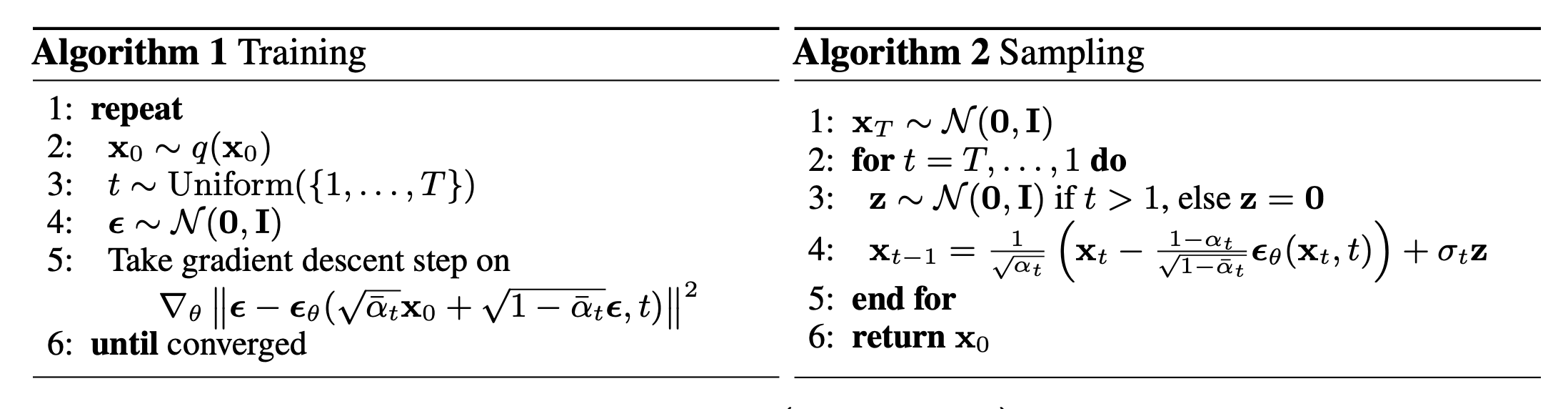
Note : DDPM は拡散モデルを実装する方法の一つに過ぎません。また、DDPM のサンプリング・アルゴリズムは完全なマルコフ連鎖を複製しています。そのため、GAN のような他の生成モデルと比較して新しいサンプルの生成は遅いです。この問題に対処するために多くの研究努力が行われてきました。一つのそのような例はノイズ除去拡散暗黙モデル、あるいは略して DDIM で、そこでは著者らはサンプリングを速くするためにマルコフ連鎖を非マルコフ過程で置き換えました。DDIM のコードサンプルは ここ で見られます。
DDPM モデルの実装は単純です。2 つの入力を取るモデルを定義します : 画像とランダムにサンプリングされた時間ステップです。各訓練ステップで、モデルを訓練するために以下の操作を実行します :
- 入力に加えるランダムノイズをサンプリングする。
- 入力をサンプリングされたノイズで拡散するために forward 過程を適用する。
- モデルは入力としてこれらのノイズのあるサンプルを受け取り、各時間ステップに対するノイズ予測を出力します。
- 真のノイズと予測されたノイズが与えられたとき、損失値を計算します。
- それから勾配を計算してモデル重みを更新します。
モデルが与えられた時間ステップでノイズのあるサンプルをノイズ除去する方法を知っていると仮定すると、純粋なノイズ分布から始めて、新しいサンプルを生成するためにこのアイデアを活用できます。
セットアップ
import math
import numpy as np
import matplotlib.pyplot as plt

# Requires TensorFlow >=2.11 for the GroupNormalization layer.
import tensorflow as tf
from tensorflow import keras
from tensorflow.keras import layers
import tensorflow_datasets as tfds
ハイパーパラメータ
batch_size = 32
num_epochs = 1  # Just for the sake of demonstration
total_timesteps = 1000
norm_groups = 8  # Number of groups used in GroupNormalization layer
learning_rate = 2e-4

img_size = 64
img_channels = 3
clip_min = -1.0
clip_max = 1.0

first_conv_channels = 64
channel_multiplier = [1, 2, 4, 8]
widths = [first_conv_channels * mult for mult in channel_multiplier]
has_attention = [False, False, True, True]
num_res_blocks = 2  # Number of residual blocks

dataset_name = "oxford_flowers102"
splits = ["train"]
データセット
花の画像を生成するために Oxford Flowers 102 データセットを使用します。前処理の視点からは、画像を望まれる画像サイズにリサイズするために中心クロッピングを使用して、ピクセル値を範囲 [-1.0, 1.0] に再スケールします。これは DDPM 論文 の著者らにより適用されたピクセル値の範囲と一致します。訓練データの増強のためには、画像を左右にランダムに反転します。
# Load the dataset
(ds,) = tfds.load(dataset_name, split=splits, with_info=False, shuffle_files=True)


def augment(img):
    """Flips an image left/right randomly."""
    return tf.image.random_flip_left_right(img)


def resize_and_rescale(img, size):
    """Resize the image to the desired size first and then
    rescale the pixel values in the range [-1.0, 1.0].

    Args:
        img: Image tensor
        size: Desired image size for resizing
    Returns:
        Resized and rescaled image tensor
    """

    height = tf.shape(img)[0]
    width = tf.shape(img)[1]
    crop_size = tf.minimum(height, width)

    img = tf.image.crop_to_bounding_box(
        img,
        (height - crop_size) // 2,
        (width - crop_size) // 2,
        crop_size,
        crop_size,
    )

    # Resize
    img = tf.cast(img, dtype=tf.float32)
    img = tf.image.resize(img, size=size, antialias=True)

    # Rescale the pixel values
    img = img / 127.5 - 1.0
    img = tf.clip_by_value(img, clip_min, clip_max)
    return img


def train_preprocessing(x):
    img = x["image"]
    img = resize_and_rescale(img, size=(img_size, img_size))
    img = augment(img)
    return img


train_ds = (
    ds.map(train_preprocessing, num_parallel_calls=tf.data.AUTOTUNE)
    .batch(batch_size, drop_remainder=True)
    .shuffle(batch_size * 2)
    .prefetch(tf.data.AUTOTUNE)
)
ガウス拡散ユティリティ
forward 過程と reverse 過程を個別のユティリティとして定義します。このユティリティの殆どのコードはわずかな変更を加えてオリジナル実装から借りています。
class GaussianDiffusion:
    """Gaussian diffusion utility.

    Args:
        beta_start: Start value of the scheduled variance
        beta_end: End value of the scheduled variance
        timesteps: Number of time steps in the forward process
    """

    def __init__(
        self,
        beta_start=1e-4,
        beta_end=0.02,
        timesteps=1000,
        clip_min=-1.0,
        clip_max=1.0,
    ):
        self.beta_start = beta_start
        self.beta_end = beta_end
        self.timesteps = timesteps
        self.clip_min = clip_min
        self.clip_max = clip_max

        # Define the linear variance schedule
        self.betas = betas = np.linspace(
            beta_start,
            beta_end,
            timesteps,
            dtype=np.float64,  # Using float64 for better precision
        )
        self.num_timesteps = int(timesteps)

        alphas = 1.0 - betas
        alphas_cumprod = np.cumprod(alphas, axis=0)
        alphas_cumprod_prev = np.append(1.0, alphas_cumprod[:-1])

        self.betas = tf.constant(betas, dtype=tf.float32)
        self.alphas_cumprod = tf.constant(alphas_cumprod, dtype=tf.float32)
        self.alphas_cumprod_prev = tf.constant(alphas_cumprod_prev, dtype=tf.float32)

        # Calculations for diffusion q(x_t | x_{t-1}) and others
        self.sqrt_alphas_cumprod = tf.constant(
            np.sqrt(alphas_cumprod), dtype=tf.float32
        )

        self.sqrt_one_minus_alphas_cumprod = tf.constant(
            np.sqrt(1.0 - alphas_cumprod), dtype=tf.float32
        )

        self.log_one_minus_alphas_cumprod = tf.constant(
            np.log(1.0 - alphas_cumprod), dtype=tf.float32
        )

        self.sqrt_recip_alphas_cumprod = tf.constant(
            np.sqrt(1.0 / alphas_cumprod), dtype=tf.float32
        )
        self.sqrt_recipm1_alphas_cumprod = tf.constant(
            np.sqrt(1.0 / alphas_cumprod - 1), dtype=tf.float32
        )

        # Calculations for posterior q(x_{t-1} | x_t, x_0)
        posterior_variance = (
            betas * (1.0 - alphas_cumprod_prev) / (1.0 - alphas_cumprod)
        )
        self.posterior_variance = tf.constant(posterior_variance, dtype=tf.float32)

        # Log calculation clipped because the posterior variance is 0 at the beginning
        # of the diffusion chain
        self.posterior_log_variance_clipped = tf.constant(
            np.log(np.maximum(posterior_variance, 1e-20)), dtype=tf.float32
        )

        self.posterior_mean_coef1 = tf.constant(
            betas * np.sqrt(alphas_cumprod_prev) / (1.0 - alphas_cumprod),
            dtype=tf.float32,
        )

        self.posterior_mean_coef2 = tf.constant(
            (1.0 - alphas_cumprod_prev) * np.sqrt(alphas) / (1.0 - alphas_cumprod),
            dtype=tf.float32,
        )

    def _extract(self, a, t, x_shape):
        """Extract some coefficients at specified timesteps,
        then reshape to [batch_size, 1, 1, 1, 1, ...] for broadcasting purposes.

        Args:
            a: Tensor to extract from
            t: Timestep for which the coefficients are to be extracted
            x_shape: Shape of the current batched samples
        """
        batch_size = x_shape[0]
        out = tf.gather(a, t)
        return tf.reshape(out, [batch_size, 1, 1, 1])

    def q_mean_variance(self, x_start, t):
        """Extracts the mean, and the variance at current timestep.

        Args:
            x_start: Initial sample (before the first diffusion step)
            t: Current timestep
        """
        x_start_shape = tf.shape(x_start)
        mean = self._extract(self.sqrt_alphas_cumprod, t, x_start_shape) * x_start
        variance = self._extract(1.0 - self.alphas_cumprod, t, x_start_shape)
        log_variance = self._extract(
            self.log_one_minus_alphas_cumprod, t, x_start_shape
        )
        return mean, variance, log_variance

    def q_sample(self, x_start, t, noise):
        """Diffuse the data.

        Args:
            x_start: Initial sample (before the first diffusion step)
            t: Current timestep
            noise: Gaussian noise to be added at the current timestep
        Returns:
            Diffused samples at timestep `t`
        """
        x_start_shape = tf.shape(x_start)
        return (
            self._extract(self.sqrt_alphas_cumprod, t, tf.shape(x_start)) * x_start
            + self._extract(self.sqrt_one_minus_alphas_cumprod, t, x_start_shape)
            * noise
        )

    def predict_start_from_noise(self, x_t, t, noise):
        x_t_shape = tf.shape(x_t)
        return (
            self._extract(self.sqrt_recip_alphas_cumprod, t, x_t_shape) * x_t
            - self._extract(self.sqrt_recipm1_alphas_cumprod, t, x_t_shape) * noise
        )

    def q_posterior(self, x_start, x_t, t):
        """Compute the mean and variance of the diffusion
        posterior q(x_{t-1} | x_t, x_0).

        Args:
            x_start: Stating point(sample) for the posterior computation
            x_t: Sample at timestep `t`
            t: Current timestep
        Returns:
            Posterior mean and variance at current timestep
        """

        x_t_shape = tf.shape(x_t)
        posterior_mean = (
            self._extract(self.posterior_mean_coef1, t, x_t_shape) * x_start
            + self._extract(self.posterior_mean_coef2, t, x_t_shape) * x_t
        )
        posterior_variance = self._extract(self.posterior_variance, t, x_t_shape)
        posterior_log_variance_clipped = self._extract(
            self.posterior_log_variance_clipped, t, x_t_shape
        )
        return posterior_mean, posterior_variance, posterior_log_variance_clipped

    def p_mean_variance(self, pred_noise, x, t, clip_denoised=True):
        x_recon = self.predict_start_from_noise(x, t=t, noise=pred_noise)
        if clip_denoised:
            x_recon = tf.clip_by_value(x_recon, self.clip_min, self.clip_max)

        model_mean, posterior_variance, posterior_log_variance = self.q_posterior(
            x_start=x_recon, x_t=x, t=t
        )
        return model_mean, posterior_variance, posterior_log_variance

    def p_sample(self, pred_noise, x, t, clip_denoised=True):
        """Sample from the diffuison model.

        Args:
            pred_noise: Noise predicted by the diffusion model
            x: Samples at a given timestep for which the noise was predicted
            t: Current timestep
            clip_denoised (bool): Whether to clip the predicted noise
                within the specified range or not.
        """
        model_mean, _, model_log_variance = self.p_mean_variance(
            pred_noise, x=x, t=t, clip_denoised=clip_denoised
        )
        noise = tf.random.normal(shape=x.shape, dtype=x.dtype)
        # No noise when t == 0
        nonzero_mask = tf.reshape(
            1 - tf.cast(tf.equal(t, 0), tf.float32), [tf.shape(x)[0], 1, 1, 1]
        )
        return model_mean + nonzero_mask * tf.exp(0.5 * model_log_variance) * noise
ネットワーク・アーキテクチャ
U-Net、元々はセマンティック・セグメンテーションのために開発されたアーキテクチャですが、それは拡散モデルの実装のために広く使用されていますが、幾つかの僅かな変更があります :
- ネットワークは 2 つの入力を受け取ります : 画像と時間ステップ
- 特定の解像度 (論文では 16×16) に到達したら畳み込みブロック間で自己アテンションを行なう。
- 重み正規化の代わりにグループ正規化
殆どのものをオリジナル論文で使用されたように実装しています。ネットワークを通して swish 活性化関数を使用しています。分散スケーリング・カーネル initializer を使用しています。
ここでの唯一の違いは GroupNormalization 層のために使用されるグループ数です。flowers データセットについては、groups=32 のデフォルト値に比べて groups=8 の値がより良い結果を生成することを見い出しました。Dropout はオプションで、過剰適合の可能性が高いところで使用されるべきです。この論文では、著者らは CIFAR10 上で訓練するときだけ dropout を使用しました。
# Kernel initializer to use
def kernel_init(scale):
    scale = max(scale, 1e-10)
    return keras.initializers.VarianceScaling(
        scale, mode="fan_avg", distribution="uniform"
    )


class AttentionBlock(layers.Layer):
    """Applies self-attention.

    Args:
        units: Number of units in the dense layers
        groups: Number of groups to be used for GroupNormalization layer
    """

    def __init__(self, units, groups=8, **kwargs):
        self.units = units
        self.groups = groups
        super().__init__(**kwargs)

        self.norm = layers.GroupNormalization(groups=groups)
        self.query = layers.Dense(units, kernel_initializer=kernel_init(1.0))
        self.key = layers.Dense(units, kernel_initializer=kernel_init(1.0))
        self.value = layers.Dense(units, kernel_initializer=kernel_init(1.0))
        self.proj = layers.Dense(units, kernel_initializer=kernel_init(0.0))

    def call(self, inputs):
        batch_size = tf.shape(inputs)[0]
        height = tf.shape(inputs)[1]
        width = tf.shape(inputs)[2]
        scale = tf.cast(self.units, tf.float32) ** (-0.5)

        inputs = self.norm(inputs)
        q = self.query(inputs)
        k = self.key(inputs)
        v = self.value(inputs)

        attn_score = tf.einsum("bhwc, bHWc->bhwHW", q, k) * scale
        attn_score = tf.reshape(attn_score, [batch_size, height, width, height * width])

        attn_score = tf.nn.softmax(attn_score, -1)
        attn_score = tf.reshape(attn_score, [batch_size, height, width, height, width])

        proj = tf.einsum("bhwHW,bHWc->bhwc", attn_score, v)
        proj = self.proj(proj)
        return inputs + proj


class TimeEmbedding(layers.Layer):
    def __init__(self, dim, **kwargs):
        super().__init__(**kwargs)
        self.dim = dim
        self.half_dim = dim // 2
        self.emb = math.log(10000) / (self.half_dim - 1)
        self.emb = tf.exp(tf.range(self.half_dim, dtype=tf.float32) * -self.emb)

    def call(self, inputs):
        inputs = tf.cast(inputs, dtype=tf.float32)
        emb = inputs[:, None] * self.emb[None, :]
        emb = tf.concat([tf.sin(emb), tf.cos(emb)], axis=-1)
        return emb


def ResidualBlock(width, groups=8, activation_fn=keras.activations.swish):
    def apply(inputs):
        x, t = inputs
        input_width = x.shape[3]

        if input_width == width:
            residual = x
        else:
            residual = layers.Conv2D(
                width, kernel_size=1, kernel_initializer=kernel_init(1.0)
            )(x)

        temb = activation_fn(t)
        temb = layers.Dense(width, kernel_initializer=kernel_init(1.0))(temb)[
            :, None, None, :
        ]

        x = layers.GroupNormalization(groups=groups)(x)
        x = activation_fn(x)
        x = layers.Conv2D(
            width, kernel_size=3, padding="same", kernel_initializer=kernel_init(1.0)
        )(x)

        x = layers.Add()([x, temb])
        x = layers.GroupNormalization(groups=groups)(x)
        x = activation_fn(x)

        x = layers.Conv2D(
            width, kernel_size=3, padding="same", kernel_initializer=kernel_init(0.0)
        )(x)
        x = layers.Add()([x, residual])
        return x

    return apply


def DownSample(width):
    def apply(x):
        x = layers.Conv2D(
            width,
            kernel_size=3,
            strides=2,
            padding="same",
            kernel_initializer=kernel_init(1.0),
        )(x)
        return x

    return apply


def UpSample(width, interpolation="nearest"):
    def apply(x):
        x = layers.UpSampling2D(size=2, interpolation=interpolation)(x)
        x = layers.Conv2D(
            width, kernel_size=3, padding="same", kernel_initializer=kernel_init(1.0)
        )(x)
        return x

    return apply


def TimeMLP(units, activation_fn=keras.activations.swish):
    def apply(inputs):
        temb = layers.Dense(
            units, activation=activation_fn, kernel_initializer=kernel_init(1.0)
        )(inputs)
        temb = layers.Dense(units, kernel_initializer=kernel_init(1.0))(temb)
        return temb

    return apply


def build_model(
    img_size,
    img_channels,
    widths,
    has_attention,
    num_res_blocks=2,
    norm_groups=8,
    interpolation="nearest",
    activation_fn=keras.activations.swish,
):
    image_input = layers.Input(
        shape=(img_size, img_size, img_channels), name="image_input"
    )
    time_input = keras.Input(shape=(), dtype=tf.int64, name="time_input")

    x = layers.Conv2D(
        first_conv_channels,
        kernel_size=(3, 3),
        padding="same",
        kernel_initializer=kernel_init(1.0),
    )(image_input)

    temb = TimeEmbedding(dim=first_conv_channels * 4)(time_input)
    temb = TimeMLP(units=first_conv_channels * 4, activation_fn=activation_fn)(temb)

    skips = [x]

    # DownBlock
    for i in range(len(widths)):
        for _ in range(num_res_blocks):
            x = ResidualBlock(
                widths[i], groups=norm_groups, activation_fn=activation_fn
            )([x, temb])
            if has_attention[i]:
                x = AttentionBlock(widths[i], groups=norm_groups)(x)
            skips.append(x)

        if widths[i] != widths[-1]:
            x = DownSample(widths[i])(x)
            skips.append(x)

    # MiddleBlock
    x = ResidualBlock(widths[-1], groups=norm_groups, activation_fn=activation_fn)(
        [x, temb]
    )
    x = AttentionBlock(widths[-1], groups=norm_groups)(x)
    x = ResidualBlock(widths[-1], groups=norm_groups, activation_fn=activation_fn)(
        [x, temb]
    )

    # UpBlock
    for i in reversed(range(len(widths))):
        for _ in range(num_res_blocks + 1):
            x = layers.Concatenate(axis=-1)([x, skips.pop()])
            x = ResidualBlock(
                widths[i], groups=norm_groups, activation_fn=activation_fn
            )([x, temb])
            if has_attention[i]:
                x = AttentionBlock(widths[i], groups=norm_groups)(x)

        if i != 0:
            x = UpSample(widths[i], interpolation=interpolation)(x)

    # End block
    x = layers.GroupNormalization(groups=norm_groups)(x)
    x = activation_fn(x)
    x = layers.Conv2D(3, (3, 3), padding="same", kernel_initializer=kernel_init(0.0))(x)
    return keras.Model([image_input, time_input], x, name="unet")
訓練
拡散モデルの訓練に対しては論文で説明されているのと同じセットアップに従います。2e-4 の学習率で Adam optimizer を使用します。0.999 の decay 因子によりモデルパラメータ上で EMA (指数平滑移動平均線) を使用します。モデルをノイズ予測ネットワークとして扱います、つまり UNet に画像のバッチと対応する時間ステップを入力して、ネットワークは予測としてノイズを出力します。
唯一の違いは、訓練の間に生成サンプルの品質を評価するためにカーネル Inception 距離 (KID) や Frechet Inception 距離 (FID) を使用しないことです。これは両方の尺度の計算が重いためで、実装の簡潔さのためにスキップされます。
Note : 損失関数としては平均二乗誤差を使用していますが、これは論文に合わせたもので、理論的にも妥当です。しかし実際には、損失関数として平均絶対誤差や Huber 損失を使用することも一般的です。
class DiffusionModel(keras.Model):
    def __init__(self, network, ema_network, timesteps, gdf_util, ema=0.999):
        super().__init__()
        self.network = network
        self.ema_network = ema_network
        self.timesteps = timesteps
        self.gdf_util = gdf_util
        self.ema = ema

    def train_step(self, images):
        # 1. Get the batch size
        batch_size = tf.shape(images)[0]

        # 2. Sample timesteps uniformly
        t = tf.random.uniform(
            minval=0, maxval=self.timesteps, shape=(batch_size,), dtype=tf.int64
        )

        with tf.GradientTape() as tape:
            # 3. Sample random noise to be added to the images in the batch
            noise = tf.random.normal(shape=tf.shape(images), dtype=images.dtype)

            # 4. Diffuse the images with noise
            images_t = self.gdf_util.q_sample(images, t, noise)

            # 5. Pass the diffused images and time steps to the network
            pred_noise = self.network([images_t, t], training=True)

            # 6. Calculate the loss
            loss = self.loss(noise, pred_noise)

        # 7. Get the gradients
        gradients = tape.gradient(loss, self.network.trainable_weights)

        # 8. Update the weights of the network
        self.optimizer.apply_gradients(zip(gradients, self.network.trainable_weights))

        # 9. Updates the weight values for the network with EMA weights
        for weight, ema_weight in zip(self.network.weights, self.ema_network.weights):
            ema_weight.assign(self.ema * ema_weight + (1 - self.ema) * weight)

        # 10. Return loss values
        return {"loss": loss}

    def generate_images(self, num_images=16):
        # 1. Randomly sample noise (starting point for reverse process)
        samples = tf.random.normal(
            shape=(num_images, img_size, img_size, img_channels), dtype=tf.float32
        )
        # 2. Sample from the model iteratively
        for t in reversed(range(0, self.timesteps)):
            tt = tf.cast(tf.fill(num_images, t), dtype=tf.int64)
            pred_noise = self.ema_network.predict(
                [samples, tt], verbose=0, batch_size=num_images
            )
            samples = self.gdf_util.p_sample(
                pred_noise, samples, tt, clip_denoised=True
            )
        # 3. Return generated samples
        return samples

    def plot_images(
        self, epoch=None, logs=None, num_rows=2, num_cols=8, figsize=(12, 5)
    ):
        """Utility to plot images using the diffusion model during training."""
        generated_samples = self.generate_images(num_images=num_rows * num_cols)
        generated_samples = (
            tf.clip_by_value(generated_samples * 127.5 + 127.5, 0.0, 255.0)
            .numpy()
            .astype(np.uint8)
        )

        _, ax = plt.subplots(num_rows, num_cols, figsize=figsize)
        for i, image in enumerate(generated_samples):
            if num_rows == 1:
                ax[i].imshow(image)
                ax[i].axis("off")
            else:
                ax[i // num_cols, i % num_cols].imshow(image)
                ax[i // num_cols, i % num_cols].axis("off")

        plt.tight_layout()
        plt.show()


# Build the unet model
network = build_model(
    img_size=img_size,
    img_channels=img_channels,
    widths=widths,
    has_attention=has_attention,
    num_res_blocks=num_res_blocks,
    norm_groups=norm_groups,
    activation_fn=keras.activations.swish,
)
ema_network = build_model(
    img_size=img_size,
    img_channels=img_channels,
    widths=widths,
    has_attention=has_attention,
    num_res_blocks=num_res_blocks,
    norm_groups=norm_groups,
    activation_fn=keras.activations.swish,
)
ema_network.set_weights(network.get_weights())  # Initially the weights are the same

# Get an instance of the Gaussian Diffusion utilities
gdf_util = GaussianDiffusion(timesteps=total_timesteps)

# Get the model
model = DiffusionModel(
    network=network,
    ema_network=ema_network,
    gdf_util=gdf_util,
    timesteps=total_timesteps,
)

# Compile the model
model.compile(
    loss=keras.losses.MeanSquaredError(),
    optimizer=keras.optimizers.Adam(learning_rate=learning_rate),
)

# Train the model
model.fit(
    train_ds,
    epochs=num_epochs,
    batch_size=batch_size,
    callbacks=[keras.callbacks.LambdaCallback(on_epoch_end=model.plot_images)],
)
31/31 [==============================] - ETA: 0s - loss: 0.7746

31/31 [==============================] - 194s 4s/step - loss: 0.7668

<keras.callbacks.History at 0x7fc9e86ce610>
結果
このモデルを V100 GPU で 800 エポック訓練し、各エポックを終えるのにおよそ 8 秒かかりました。これらの重みをここでロードして、純粋なノイズから始めて幾つかサンプルを生成します。
!curl -LO https://github.com/AakashKumarNain/ddpms/releases/download/v3.0.0/checkpoints.zip
!unzip -qq checkpoints.zip
# Load the model weights
model.ema_network.load_weights("checkpoints/diffusion_model_checkpoint")

# Generate and plot some samples
model.plot_images(num_rows=4, num_cols=8)
  % Total    % Received % Xferd  Average Speed   Time    Time     Time  Current
                                 Dload  Upload   Total   Spent    Left  Speed
  0     0    0     0    0     0      0      0 --:--:-- --:--:-- --:--:--     0
100  222M  100  222M    0     0  16.0M      0  0:00:13  0:00:13 --:--:-- 14.7M

まとめ
拡散モデルを DDPM 論文の著者による実装と正確に同じ流儀で実装して訓練することに成功しました。オリジナルの実装は ここ で見つけられます。
モデルを改良するために試せる 2,3 のことがあります :
- 各ブロックの width を大きくする。より大きいモデルはノイズ除去をより少ないエポックで学習できます、過剰適合に注意する必要はあるかもしれませんが。
- 分散スケジューリングのために線形スケジュールを実装しました。コサインスケジューリングのような他のスキームを実装して性能を比較することができます。
リファレンス
- Denoising Diffusion Probabilistic Models
- 著者の実装
- A deep dive into DDPMs
- Denoising Diffusion Implicit Models
- Annotated Diffusion Model
- AIAIART
以上